Control Variates for Coupon-Bond Pricing under the Black–Karasinski Model 2

Introduction

지난 글에서는 Black–Karasinski(BK)와 Vasicek 모델의 수학적 구조, 할인계수, 쿠폰 채권의 Monte Carlo 가격 추정과 Control Variates의 기본 원리를 정리했다.

이번 글에서는 앞에서 다룬 내용을 Python으로 구현하고 실제 출력값을 확인한다. 먼저 Vasicek의 해석적 가격과 Monte Carlo 추정값을 비교하여 계산을 검증하고, BK 채권 가격을 추정한다. 이후 Vasicek과 BK 경로 기반 통제변량을 각각 적용해 표준오차와 VRF를 비교한다. 마지막으로 통제변량의 기대값이 잘못되었을 때 결과에 어떤 문제가 발생하는지도 확인한다.

Parameters

구분	파라미터	값
BK	κ, θ, r₀	0.8, ln(0.03), 0.03
BK	σ	0.2, 0.5
Vasicek (기본값)	α, β, η, r₀ᵛ	0.8, 0.03, 0.01, 0.03
Bond	T, C, Principal	5 years, 0.04, 1
Simulation	Δt, N	1/52, 20,000
CV pre-run	N̂	2,000 (별도 표본)

BK에서는 σ 값을 두 가지로 나누어 같은 가격 추정 방법의 성능을 비교한다. σ를 낮춰 SE를 줄이는 것이 아니라 σ를 고정한 채 통제변량으로 SE를 줄이는 것이 목적이다.

---

Part A: Plain Monte Carlo in the Vasicek Model

Vasicek 모델은 해석적 채권 가격을 구할 수 있어 MC 시뮬레이션을 검증할 기준으로 사용한다. 표본오차와 이산화 오차는 구분해서 해석해야 한다.

Task 1. Vasicek Plain Monte Carlo

Vasicek의 금리를 Euler 방법으로 생성하고 적분 금리를 사다리꼴 공식으로 근사한다. 쿠폰 지급 시점마다 할인계수를 적용하여 경로별 가격을 구한 뒤, 그 평균과 표준오차를 계산한다.

Python Implementation (Notebook 셀 2)

import numpy as np

# 1. Parameters
alpha = 0.8
beta = 0.03
eta = 0.01
r0 = 0.03

T = 5
C = 0.04
principal = 1.0

dt = 1 / 52
N = 20000
seed = 2026

# 2. Vasicek Monte Carlo simulation
def vasicek_mc(N, dt, seed=2026):
    rng = np.random.default_rng(seed)

    M = round(T / dt)
    dt = T / M
    sqrt_dt = np.sqrt(dt)

    rates = np.full(N, r0, dtype=float)
    integrated_rates = np.zeros(N)
    payoffs = np.zeros(N)

    steps_per_year = M // T

    for k in range(1, M + 1):

        # Euler scheme
        Z = rng.standard_normal(N)

        next_rates = (
            rates
            + alpha * (beta - rates) * dt
            + eta * sqrt_dt * Z
        )

        # Trapezoidal rule
        integrated_rates += (
            0.5 * (rates + next_rates) * dt
        )

        rates = next_rates

        # Annual coupon payments
        if k % steps_per_year == 0:
            year = k // steps_per_year

            cashflow = C

            if year == T:
                cashflow += principal

            discount_factor = np.exp(-integrated_rates)

            payoffs += cashflow * discount_factor

    # Plain Monte Carlo price
    mc_price = np.mean(payoffs)

    # Estimated standard error
    sample_std = np.std(payoffs, ddof=1)
    se = sample_std / np.sqrt(N)

    return mc_price, se, payoffs


mc_price, se, payoffs = vasicek_mc(N, dt, seed)

print("=== Task 1: Vasicek Plain Monte Carlo ===")
print(f"Number of paths: {N:,}")
print(f"Time step: {dt:.8f}")
print(f"MC bond price: {mc_price:.8f}")
print(f"Standard error: {se:.8f}")

저장된 실행 결과

=== Task 1: Vasicek Plain Monte Carlo ===
Number of paths: 20,000
Time step: 0.01923077
MC bond price: 1.04383592
Standard error: 0.00015148

Task 2. Vasicek 해석적 가격과 비교

Vasicek은 해석적 채권 가격 공식이 있으므로 MC 결과와 비교할 수 있다. 가격 차이가 표본오차 크기에 비추어 합리적인지 확인하고 Δt를 바꿔 이산화 오차 가능성을 함께 살펴본다.

Python Implementation (Notebook 셀 4)

# 3. Analytical Vasicek zero-coupon bond price
def vasicek_zero_coupon(t):
    B = -np.expm1(-alpha * t) / alpha

    A = (
        (beta - eta**2 / (2 * alpha**2)) * (B - t)
        - (eta**2 / (4 * alpha)) * B**2
    )

    return np.exp(A - B * r0)


# 4. Analytical coupon-bond price
analytical_price = 0.0

for year in range(1, T + 1):
    cashflow = C

    if year == T:
        cashflow += principal

    analytical_price += (
        cashflow * vasicek_zero_coupon(year)
    )


# 5. Comparison with Monte Carlo
difference = mc_price - analytical_price
absolute_error = abs(difference)
error_in_se = absolute_error / se

print("=== Task 2: Analytical Comparison ===")
print(f"Analytical price: {analytical_price:.8f}")
print(f"MC price:         {mc_price:.8f}")
print(f"Standard error:   {se:.8f}")
print(f"Absolute error:   {absolute_error:.8f}")
print(f"Error / SE:       {error_in_se:.4f}")


# 6. Finer time step
dt_fine = 1 / 252

mc_fine, se_fine, _ = vasicek_mc(
    N, dt_fine, seed
)

print("\n=== Time Step Comparison ===")
print(f"dt = 1/52  : {mc_price:.8f}, SE = {se:.8f}")
print(f"dt = 1/252 : {mc_fine:.8f}, SE = {se_fine:.8f}")
print(f"Analytical: {analytical_price:.8f}")

저장된 실행 결과

=== Task 2: Analytical Comparison ===
Analytical price: 1.04389268
MC price:         1.04383592
Standard error:   0.00015148
Absolute error:   0.00005676
Error / SE:       0.3747

=== Time Step Comparison ===
dt = 1/52  : 1.04383592, SE = 0.00015148
dt = 1/252 : 1.04382200, SE = 0.00015169
Analytical: 1.04389268

Python Implementation (Notebook 셀 5)

# Basic numerical validation

# Test 1: The simulation generates N payoffs
assert len(payoffs) == N

# Test 2: All simulated prices are finite
assert np.all(np.isfinite(payoffs))

# Test 3: The discounting produces positive path values
assert np.all(payoffs > 0)

# Test 4: The estimated standard error is positive
assert se > 0

# Test 5: The analytic zero-coupon price at t=0 equals 1
assert np.isclose(
    vasicek_zero_coupon(0),
    1.0,
    atol=1e-12
)

print("All basic validation tests passed.")

저장된 실행 결과

All basic validation tests passed.

Part B: Plain Monte Carlo in the BK Model

BK에서는 로그 금리를 Euler로 생성한 다음 지수함수로 실제 금리를 구하고, 할인계수로 쿠폰 채권의 현재가치를 계산한다.

Task 3. BK Plain Monte Carlo

이번에는 BK 로그 금리에 Euler 방법을 적용한다. 실제 금리는 지수함수로 계산하고 두 가지 변동성 σ=0.2, 0.5에서 가격과 SE를 비교한다.

Python Implementation (Notebook 셀 7)

import numpy as np

# 1. BK parameters
kappa = 0.8
theta = np.log(0.03)
r0_bk = 0.03
sigmas = [0.2, 0.5]

# 2. Bond and simulation parameters
T = 5
C = 0.04
principal = 1.0

N = 20000
dt = 1 / 52
seed = 2026


def bk_mc(sigma, N=20000, dt=1/52, seed=2026):
    rng = np.random.default_rng(seed)

    M = round(T / dt)
    dt = T / M
    sqrt_dt = np.sqrt(dt)
    steps_per_year = M // T

    # Initial log short rates
    x = np.full(N, np.log(r0_bk), dtype=float)

    integrated_rates = np.zeros(N)
    payoffs = np.zeros(N)

    for k in range(1, M + 1):

        # Generate Brownian increments
        Z = rng.standard_normal(N)

        # Euler scheme for log short rates
        x_next = (
            x
            + kappa * (theta - x) * dt
            + sigma * sqrt_dt * Z
        )

        # Convert log rates to short rates
        r_current = np.exp(x)
        r_next = np.exp(x_next)

        # Trapezoidal integration
        integrated_rates += (
            0.5 * (r_current + r_next) * dt
        )

        x = x_next

        # Annual coupon payments
        if k % steps_per_year == 0:
            year = k // steps_per_year

            cashflow = C

            if year == T:
                cashflow += principal

            discount_factor = np.exp(-integrated_rates)

            payoffs += cashflow * discount_factor

    # Monte Carlo estimate
    mc_price = np.mean(payoffs)

    # Estimated standard error
    sample_std = np.std(payoffs, ddof=1)
    se = sample_std / np.sqrt(N)

    return mc_price, se, payoffs


# 3. Results for both volatility values
results_bk = {}

for sigma in sigmas:
    price, se, payoffs = bk_mc(
        sigma=sigma,
        N=N,
        dt=dt,
        seed=seed
    )

    results_bk[sigma] = {
        "price": price,
        "se": se,
        "payoffs": payoffs
    }

    print(f"=== BK Model: sigma = {sigma} ===")
    print(f"MC bond price: {price:.8f}")
    print(f"Standard error: {se:.8f}")
    print()

저장된 실행 결과

=== BK Model: sigma = 0.2 ===
MC bond price: 1.04212403
Standard error: 0.00009197

=== BK Model: sigma = 0.5 ===
MC bond price: 1.03400908
Standard error: 0.00024446

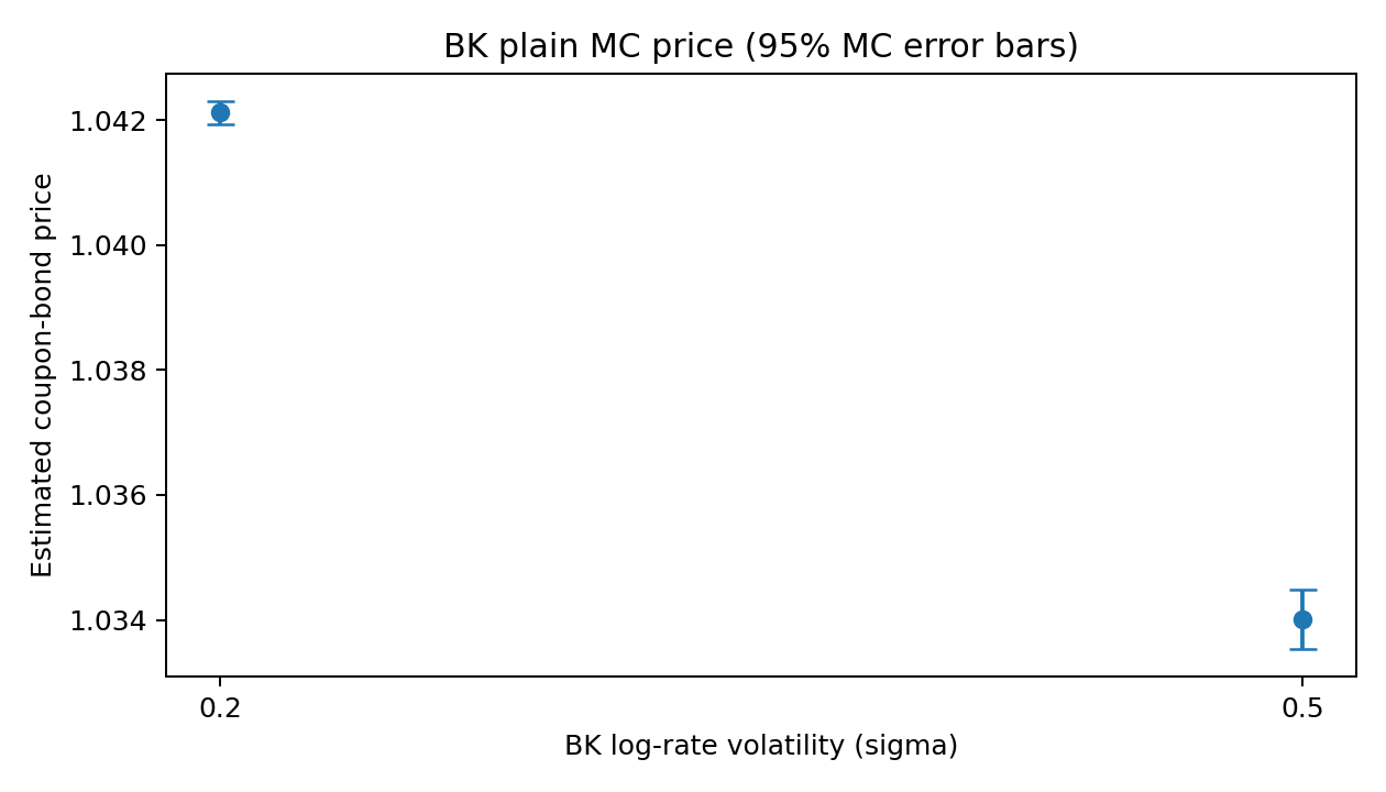
Figure 1. BK 변동성별 MC 채권 가격. 오차 막대는 ±1.96 SE를 나타낸다.

Python Implementation (Notebook 셀 8)

# Validation for Part B

# Test 1: Correct number of simulated payoffs
for sigma in sigmas:
    payoffs = results_bk[sigma]["payoffs"]
    assert len(payoffs) == N

# Test 2: All payoffs are finite and positive
for sigma in sigmas:
    payoffs = results_bk[sigma]["payoffs"]
    assert np.all(np.isfinite(payoffs))
    assert np.all(payoffs > 0)

# Test 3: Standard errors are finite and positive
for sigma in sigmas:
    se = results_bk[sigma]["se"]
    assert np.isfinite(se)
    assert se > 0

# Test 4: Deterministic case (sigma = 0)
# Since theta = log(r0), the rate stays at r0.
price_zero, se_zero, _ = bk_mc(
    sigma=0.0,
    N=100,
    dt=dt,
    seed=seed
)

expected_price = (
    sum(C * np.exp(-r0_bk * year)
        for year in range(1, T + 1))
    + principal * np.exp(-r0_bk * T)
)

assert np.isclose(
    price_zero,
    expected_price,
    atol=1e-12
)
assert se_zero < 1e-12

print("All Part B validation tests passed.")

저장된 실행 결과

All Part B validation tests passed.

Part C: Vasicek Control Variates

BK와 Vasicek에 같은 Gaussian increments를 사용한다. Vasicek 무이표채권과 쿠폰 채권의 기대값을 이용해 BK 추정량을 보정하고, 보정 계수는 독립 pre-run에서 추정한다.

Part C 개요

BK와 Vasicek에 같은 표준정규 난수를 사용한다. Vasicek의 무이표채권과 쿠폰 채권을 통제변량으로 사용해 BK 가격 추정의 분산이 얼마나 감소하는지 확인한다.

Python Implementation (Notebook 셀 10)

import numpy as np
import matplotlib.pyplot as plt

# BK parameters
KAPPA = 0.8
THETA = np.log(0.03)
R0 = 0.03
SIGMAS = (0.2, 0.5)

# Bond and simulation parameters
T = 5
COUPON = 0.04
N = 20000
N_PILOT = 2000
DT = 1 / 52
SEED = 2026

# Initial Vasicek parameters
BASE_PARAMS = (0.8, 0.03, 0.01)


def generate_normals(n, dt, seed):
    m = round(T / dt)

    assert np.isclose(m * dt, T)
    assert m % T == 0

    rng = np.random.default_rng(seed)
    return rng.standard_normal((m, n))


def simulate_joint(z, sigma, alpha, beta, eta, dt=DT):
    """
    Simulate BK and Vasicek models using identical Gaussian increments.
    Return BK coupon payoff, Vasicek zero-coupon control,
    and Vasicek coupon-bond control.
    """
    m, n = z.shape
    steps_per_year = m // T

    x = np.full(n, np.log(R0), dtype=float)
    v = np.full(n, R0, dtype=float)

    I_bk = np.zeros(n)
    I_vas = np.zeros(n)

    Y = np.zeros(n)
    X_coupon = np.zeros(n)

    sqrt_dt = np.sqrt(dt)

    for k in range(1, m + 1):
        zk = z[k - 1]

        # BK Euler scheme: simulate the log short rate
        x_next = (
            x
            + KAPPA * (THETA - x) * dt
            + sigma * sqrt_dt * zk
        )

        # Vasicek Euler scheme: same Gaussian increments
        v_next = (
            v
            + alpha * (beta - v) * dt
            + eta * sqrt_dt * zk
        )

        # Integrated rates using the trapezoidal rule
        I_bk += 0.5 * (np.exp(x) + np.exp(x_next)) * dt
        I_vas += 0.5 * (v + v_next) * dt

        x = x_next
        v = v_next

        if k % steps_per_year == 0:
            cashflow = COUPON + (1.0 if k == m else 0.0)

            Y += cashflow * np.exp(-I_bk)
            X_coupon += cashflow * np.exp(-I_vas)

    X_zcb = np.exp(-I_vas)

    return Y, X_zcb, X_coupon


# Separate Gaussian samples for coefficient estimation and pricing
z_pilot = generate_normals(N_PILOT, DT, SEED + 1)
z_pricing = generate_normals(N, DT, SEED)

print("Part C simulation functions ready.")
print(f"Pilot paths: {N_PILOT}")
print(f"Pricing paths: {N}")

저장된 실행 결과

Part C simulation functions ready.
Pilot paths: 2000
Pricing paths: 20000

Task 4. Vasicek 통제변량 두 종류

통제변량은 Vasicek 만기 할인계수와 Vasicek 쿠폰 채권 가치이다. 별도 2,000개 경로로 보정 계수를 추정한 뒤 20,000개 가격 경로에 적용한다. 기대값은 실제 Euler·사다리꼴 방식으로 생성한 통제변량과 일치하도록 계산한다.

Python Implementation (Notebook 셀 12)

def vasicek_control_expectations(alpha, beta, eta, dt=DT):
    """
    Exact expectations of the discretized Vasicek controls.

    Euler rates and trapezoidal integrated rates are Gaussian.
    Their means and covariance matrices are propagated exactly.
    """
    m = round(T / dt)
    steps_per_year = m // T

    # State = [short rate, integrated short rate]
    mean = np.array([R0, 0.0])
    cov = np.zeros((2, 2))

    a = 1 - alpha * dt
    b = alpha * beta * dt
    q = eta * np.sqrt(dt)

    A = np.array([
        [a, 0.0],
        [0.5 * dt * (1 + a), 1.0]
    ])

    shift = np.array([b, 0.5 * dt * b])
    noise = np.array([q, 0.5 * dt * q])

    coupon_expectation = 0.0

    for k in range(1, m + 1):
        mean = A @ mean + shift
        cov = A @ cov @ A.T + np.outer(noise, noise)

        if k % steps_per_year == 0:
            cashflow = COUPON + (1.0 if k == m else 0.0)

            # For Gaussian I: E[exp(-I)] = exp(-E[I] + Var(I)/2)
            expected_discount = np.exp(
                -mean[1] + 0.5 * cov[1, 1]
            )

            coupon_expectation += cashflow * expected_discount

    zcb_expectation = np.exp(
        -mean[1] + 0.5 * cov[1, 1]
    )

    return zcb_expectation, coupon_expectation


def control_variate(y_pilot, x_pilot, y_price, x_price, mu):
    """
    Fit the control coefficient on the pilot sample
    and evaluate the CV estimator on independent pricing paths.
    """
    x_pilot = np.asarray(x_pilot)
    x_price = np.asarray(x_price)

    # Sample covariance / sample variance
    nu = (
        np.cov(x_pilot, y_pilot, ddof=1)[0, 1]
        / np.var(x_pilot, ddof=1)
    )

    y_cv = y_price - nu * (x_price - mu)

    price = np.mean(y_cv)
    se = np.std(y_cv, ddof=1) / np.sqrt(len(y_cv))

    vrf = (
        np.var(y_price, ddof=1)
        / np.var(y_cv, ddof=1)
    )

    return {
        "price": float(price),
        "se": float(se),
        "nu": float(nu),
        "vrf": float(vrf)
    }


def evaluate_controls(sigma, params, z_pilot, z_pricing):
    alpha, beta, eta = params

    Y_pilot, Xz_pilot, Xc_pilot = simulate_joint(
        z_pilot, sigma, alpha, beta, eta
    )

    Y, Xz, Xc = simulate_joint(
        z_pricing, sigma, alpha, beta, eta
    )

    mu_z, mu_c = vasicek_control_expectations(
        alpha, beta, eta
    )

    zcb_result = control_variate(
        Y_pilot, Xz_pilot, Y, Xz, mu_z
    )

    coupon_result = control_variate(
        Y_pilot, Xc_pilot, Y, Xc, mu_c
    )

    plain_price = np.mean(Y)
    plain_se = np.std(Y, ddof=1) / np.sqrt(len(Y))

    return {
        "plain_price": float(plain_price),
        "plain_se": float(plain_se),
        "zcb": zcb_result,
        "coupon": coupon_result
    }


print("Control-variate functions ready.")

Control-variate functions ready.

Python Implementation (Notebook 셀 13)

task4_results = {}

for sigma in SIGMAS:
    result = evaluate_controls(
        sigma,
        BASE_PARAMS,
        z_pilot,
        z_pricing
    )

    task4_results[sigma] = result

    print(f"\n=== BK sigma = {sigma} ===")
    print(f"Plain MC price: {result['plain_price']:.8f}")
    print(f"Plain MC SE:    {result['plain_se']:.8f}")

    for name in ["zcb", "coupon"]:
        r = result[name]

        print(f"\nControl: {name}")
        print(f"CV price: {r['price']:.8f}")
        print(f"CV SE:    {r['se']:.8f}")
        print(f"nu:       {r['nu']:.6f}")
        print(f"VRF:      {r['vrf']:.4f}")

저장된 실행 결과

=== BK sigma = 0.2 ===
Plain MC price: 1.04212403
Plain MC SE:    0.00009197

Control: zcb
CV price: 1.04216099
CV SE:    0.00000884
nu:       0.672563
VRF:      108.3568

Control: coupon
CV price: 1.04215894
CV SE:    0.00000816
nu:       0.604759
VRF:      127.1633

=== BK sigma = 0.5 ===
Plain MC price: 1.03400908
Plain MC SE:    0.00024446

Control: zcb
CV price: 1.03410593
CV SE:    0.00004926
nu:       1.762282
VRF:      24.6262

Control: coupon
CV price: 1.03410052
CV SE:    0.00004851
nu:       1.584209
VRF:      25.3936

Task 4 해석. 두 통제변량 모두 SE를 낮췄으며 이 실험에서는 쿠폰 채권 통제변량의 VRF가 조금 더 높다. 동일한 지급 구조가 BK 채권 가치의 변동을 더 잘 설명할 수 있기 때문이다.

Task 5. Vasicek 파라미터 매칭

BK의 금리 동역학을 장기 금리 근방에서 1차로 근사하면 α≈κ, β≈exp(θ), η≈σ exp(θ)라는 규칙을 얻는다. 이는 Itô 보정항과 고차항을 무시한 국소 근사이며 두 모형이 정확히 같다는 뜻은 아니다.

Python Implementation (Notebook 셀 16)

def match_vasicek_parameters(sigma):
    r_bar = np.exp(THETA)

    alpha = KAPPA
    beta = r_bar
    eta = sigma * r_bar

    return alpha, beta, eta


matched_params = {}

for sigma in SIGMAS:
    params = match_vasicek_parameters(sigma)
    matched_params[sigma] = params

    alpha, beta, eta = params

    print(f"BK sigma = {sigma}")
    print(f"alpha = {alpha:.6f}")
    print(f"beta  = {beta:.6f}")
    print(f"eta   = {eta:.6f}")
    print()

저장된 실행 결과

BK sigma = 0.2
alpha = 0.800000
beta  = 0.030000
eta   = 0.006000

BK sigma = 0.5
alpha = 0.800000
beta  = 0.030000
eta   = 0.015000

Task 6. VRF를 높이는 파라미터 탐색

α와 η를 격자 형태로 바꾸되 모든 조합에서 같은 난수를 사용하여 비교한다. 두 통제변량 각각의 VRF 히트맵을 생성하고 β를 바꿨을 때의 영향도 확인한다. 결과는 지정한 격자 내에서의 최선일 뿐 전역 최적을 보장하지 않는다.

Python Implementation (Notebook 셀 18)

# Search ranges
alpha_grid = np.linspace(0.35, 1.65, 9)
eta_grid = np.linspace(0.002, 0.032, 11)

beta_search = 0.03

# Common random numbers for the entire grid
z_search = generate_normals(
    n=2000,
    dt=DT,
    seed=123456
)


def calculate_grid_vrf(sigma):
    vrf_zcb = np.zeros(
        (len(eta_grid), len(alpha_grid))
    )

    vrf_coupon = np.zeros_like(vrf_zcb)

    for i, eta in enumerate(eta_grid):
        for j, alpha in enumerate(alpha_grid):

            Y, Xz, Xc = simulate_joint(
                z_search,
                sigma,
                alpha,
                beta_search,
                eta
            )

            # Optimal scalar CV variance reduction
            corr_z = np.corrcoef(Y, Xz)[0, 1]
            corr_c = np.corrcoef(Y, Xc)[0, 1]

            vrf_zcb[i, j] = 1 / (1 - corr_z**2)
            vrf_coupon[i, j] = 1 / (1 - corr_c**2)

    return vrf_zcb, vrf_coupon


grid_results = {}

for sigma in SIGMAS:
    grid_results[sigma] = calculate_grid_vrf(sigma)

    print(f"Grid search completed: sigma = {sigma}")

저장된 실행 결과

Grid search completed: sigma = 0.2
Grid search completed: sigma = 0.5

Python Implementation (Notebook 셀 19)

%matplotlib inline

import matplotlib.pyplot as plt

for sigma in SIGMAS:
    vrf_zcb, vrf_coupon = grid_results[sigma]

    fig, axes = plt.subplots(1, 2, figsize=(12, 4.5))

    controls = [
        ("Vasicek ZCB control", vrf_zcb),
        ("Vasicek coupon-bond control", vrf_coupon)
    ]

    for ax, (title, values) in zip(axes, controls):
        im = ax.imshow(
            values,
            origin="lower",
            aspect="auto",
            extent=[
                alpha_grid[0],
                alpha_grid[-1],
                eta_grid[0],
                eta_grid[-1]
            ]
        )

        ax.set_title(title)
        ax.set_xlabel("alpha")
        ax.set_ylabel("eta")

        fig.colorbar(im, ax=ax, label="VRF")

    fig.suptitle(f"BK sigma = {sigma}")

    plt.tight_layout()

    filename = f"vrf_heatmap_sigma_{sigma}.png"
    plt.savefig(filename, dpi=200, bbox_inches="tight")

    plt.show()

    print(f"Saved: {filename}")

저장된 실행 결과

Saved: vrf_heatmap_sigma_0.2.png
Saved: vrf_heatmap_sigma_0.5.png

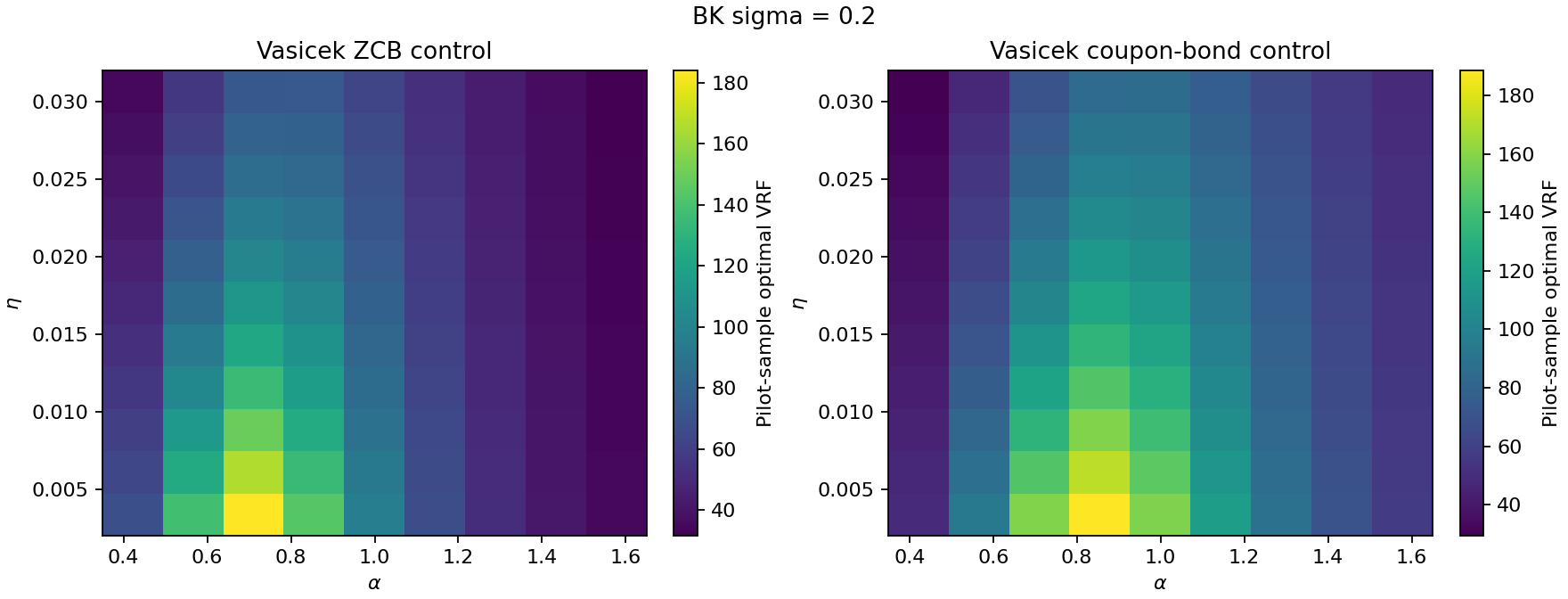
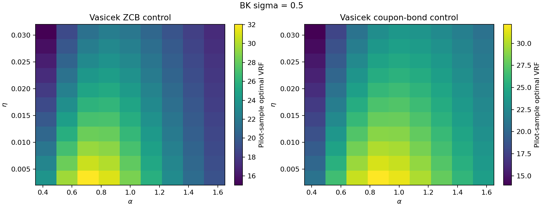
Figure 2–3. Vasicek 파라미터 α, η에 따른 VRF. 히트맵은 탐색 표본의 결과이며 전역 최적값은 아니다.

Python Implementation (Notebook 셀 20)

# Investigate the effect of beta
beta_values = [0.01, 0.03, 0.05]

alpha = 0.8
eta = 0.015
sigma = 0.5

z_beta = generate_normals(
    n=20000,
    dt=DT,
    seed=SEED + 5
)

for beta in beta_values:
    Y, Xz, Xc = simulate_joint(
        z_beta,
        sigma,
        alpha,
        beta,
        eta
    )

    corr_z = np.corrcoef(Y, Xz)[0, 1]
    corr_c = np.corrcoef(Y, Xc)[0, 1]

    vrf_z = 1 / (1 - corr_z**2)
    vrf_c = 1 / (1 - corr_c**2)

    print(f"beta = {beta:.2f}")
    print(f"ZCB VRF:    {vrf_z:.4f}")
    print(f"Coupon VRF: {vrf_c:.4f}")
    print()

저장된 실행 결과

beta = 0.01
ZCB VRF:    24.8902
Coupon VRF: 25.6588

beta = 0.03
ZCB VRF:    24.8902
Coupon VRF: 25.6574

beta = 0.05
ZCB VRF:    24.8902
Coupon VRF: 25.6528

Task 6 해석. β를 바꿔도 Vasicek ZCB 통제변량의 최적 스칼라 VRF는 변하지 않았고, 쿠폰 채권의 VRF는 소폭 달라졌다. 만기 하나의 할인계수는 β 변화에 대해 공통 배수로 변하지만 쿠폰 채권은 여러 만기의 현금흐름을 더하기 때문이다.

Task 7. 파라미터 선택에 따른 성능 비교

기본값, Task 5의 근사값, Task 6의 격자 탐색값을 별도 가격 표본으로 평가한다. 가격·SE·ν̂·VRF를 함께 출력하고 근사 규칙이 반드시 최고 VRF를 주는 것은 아닌지 확인한다.

Python Implementation (Notebook 셀 23)

task7_results = []

for sigma in SIGMAS:

    # Baseline and Task 5 matching
    baseline = BASE_PARAMS
    matched = matched_params[sigma]

    for control_index, control_name in [
        (0, "zcb"),
        (1, "coupon")
    ]:
        # Best parameter combination from Task 6 grid
        vrf_grid = grid_results[sigma][control_index]

        best_i, best_j = np.unravel_index(
            np.argmax(vrf_grid),
            vrf_grid.shape
        )

        best_params = (
            float(alpha_grid[best_j]),
            beta_search,
            float(eta_grid[best_i])
        )

        choices = {
            "Baseline": baseline,
            "Matched": matched,
            "Grid best": best_params
        }

        print(f"\nBK sigma = {sigma}, control = {control_name}")

        for choice_name, params in choices.items():
            results = evaluate_controls(
                sigma,
                params,
                z_pilot,
                z_pricing
            )

            r = results[control_name]

            task7_results.append({
                "sigma": sigma,
                "control": control_name,
                "choice": choice_name,
                "alpha": params[0],
                "beta": params[1],
                "eta": params[2],
                "price": r["price"],
                "se": r["se"],
                "nu": r["nu"],
                "vrf": r["vrf"]
            })

            print(
                f"{choice_name:10s} "
                f"params={params} "
                f"price={r['price']:.8f} "
                f"SE={r['se']:.8f} "
                f"nu={r['nu']:.5f} "
                f"VRF={r['vrf']:.2f}"
            )

저장된 실행 결과

BK sigma = 0.2, control = zcb
Baseline   params=(0.8, 0.03, 0.01) price=1.04216099 SE=0.00000884 nu=0.67256 VRF=108.36
Matched    params=(0.8, 0.029999999999999995, 0.005999999999999999) price=1.04216098 SE=0.00000837 nu=1.12178 VRF=120.78
Grid best  params=(0.6749999999999999, 0.03, 0.002) price=1.04215872 SE=0.00000730 nu=2.98761 VRF=158.51

BK sigma = 0.2, control = coupon
Baseline   params=(0.8, 0.03, 0.01) price=1.04215894 SE=0.00000816 nu=0.60476 VRF=127.16
Matched    params=(0.8, 0.029999999999999995, 0.005999999999999999) price=1.04215895 SE=0.00000766 nu=1.00866 VRF=144.01
Grid best  params=(0.8374999999999999, 0.03, 0.002) price=1.04215954 SE=0.00000721 nu=3.13084 VRF=162.75

BK sigma = 0.5, control = zcb
Baseline   params=(0.8, 0.03, 0.01) price=1.03410593 SE=0.00004926 nu=1.76228 VRF=24.63
Matched    params=(0.8, 0.029999999999999995, 0.014999999999999998) price=1.03410588 SE=0.00005083 nu=1.17259 VRF=23.13
Grid best  params=(0.6749999999999999, 0.03, 0.002) price=1.03410006 SE=0.00004620 nu=7.83555 VRF=28.00

BK sigma = 0.5, control = coupon
Baseline   params=(0.8, 0.03, 0.01) price=1.03410052 SE=0.00004851 nu=1.58421 VRF=25.39
Matched    params=(0.8, 0.029999999999999995, 0.014999999999999998) price=1.03410040 SE=0.00005007 nu=1.05416 VRF=23.84
Grid best  params=(0.8374999999999999, 0.03, 0.002) price=1.03410222 SE=0.00004607 nu=8.21159 VRF=28.15

Task 7 해석. 이번 실험에서 격자 탐색값이 더 높은 VRF를 보였지만 η가 탐색 범위의 하한에 있어 최적값 해석에는 주의가 필요하다. ν̂는 통제변량의 단위와 스케일에 따라 달라지므로 값의 크기만으로 성능을 판단할 수 없다.

Part C Validation

통제변량 표본평균이 계산된 기대값으로부터 4 SE 안에 있는지 확인하고 가격·SE·VRF가 유한한지 테스트한다. 이 기본 테스트만으로 기대값 공식의 모든 오류를 배제할 수는 없다.

Python Implementation (Notebook 셀 26)

for sigma in SIGMAS:
    alpha, beta, eta = BASE_PARAMS

    Y, Xz, Xc = simulate_joint(
        z_pricing,
        sigma,
        alpha,
        beta,
        eta
    )

    mu_z, mu_c = vasicek_control_expectations(
        alpha,
        beta,
        eta
    )

    # Finite and positive simulated payoffs
    assert np.all(np.isfinite(Y))
    assert np.all(np.isfinite(Xz))
    assert np.all(np.isfinite(Xc))

    assert np.all(Y > 0)
    assert np.all(Xz > 0)
    assert np.all(Xc > 0)

    # Control expectation checks
    se_z = np.std(Xz, ddof=1) / np.sqrt(N)
    se_c = np.std(Xc, ddof=1) / np.sqrt(N)

    assert abs(np.mean(Xz) - mu_z) < 4 * se_z
    assert abs(np.mean(Xc) - mu_c) < 4 * se_c

    # CV output checks
    results = task4_results[sigma]

    for control_name in ["zcb", "coupon"]:
        r = results[control_name]

        assert np.isfinite(r["price"])
        assert np.isfinite(r["se"])
        assert np.isfinite(r["nu"])
        assert np.isfinite(r["vrf"])

        assert r["se"] > 0
        assert r["vrf"] > 0

    print(f"BK sigma={sigma}: validation passed")

print("All Part C basic validation tests passed.")

저장된 실행 결과

BK sigma=0.2: validation passed
BK sigma=0.5: validation passed
All Part C basic validation tests passed.

Part C 정리

Vasicek 두 종류의 통제변량을 비교하고, 모델 근사 규칙과 수치 탐색을 통해 보정 성능이 파라미터에 따라 어떻게 달라지는지 확인했다.

Part D: Controls Built from the BK Path

두 번째 모델 없이 BK 적분 금리의 함수 자체를 통제변량으로 사용한다. 특히 2차 항까지 활용하여 할인계수의 비선형성을 근사한다.

Task 8. BK 적분 금리 통제변량의 기대값

Part D에서는 다른 금리 모델 대신 BK 적분 금리 I(t) 자체를 사용한다. 할인계수의 2차 근사 exp(-I) ≈ 1 − I + I²/2를 바탕으로 X₁ = Σ cᵢI(tᵢ), X₂ = Σ cᵢI(tᵢ)²를 구성한다.

기대값 유도

BK 로그 금리 x(t)는 Gaussian 과정이고 실제 금리는 exp(x(t))이므로 금리의 1차·2차 모멘트를 계산할 수 있다. 먼저 연속시간 기대값을 유도하고 실제 CV 구현에서는 Euler·Trapezoidal 방식과 일치하는 이산시간 기대값을 사용한다.

The log short rate follows an Ornstein–Uhlenbeck process, which is Gaussian.

Assuming that the initial log rate x_0 is deterministic, its mean is:

Its covariance function is:

Since r_t = exp(x_t), the short rate follows a lognormal distribution at each fixed time.

Therefore,

The integrated short rate is:

Its first moment is:

To derive its second moment, we write:

Because the log rates are jointly Gaussian,

Thus, the expectations of the two coupon-weighted controls are:

These expressions provide the theoretical expectations under the continuous-time BK model.

However, our Monte Carlo implementation uses the Euler scheme and trapezoidal integration. Therefore, the simulated integrated rate is a discretized approximation.

For the control-variate calculation, we will derive its exact discrete-time moments using the Gaussian structure of the Euler log-rate process.

This ensures that the control expectations correspond to the quantities actually simulated.

Python Implementation (Notebook 셀 30)

import numpy as np
import matplotlib.pyplot as plt

# Part D parameters
D_KAPPA = 0.8
D_THETA = np.log(0.03)
D_R0 = 0.03

D_SIGMAS = (0.2, 0.5)

D_T = 5
D_COUPON = 0.04
D_PRINCIPAL = 1.0

D_DT = 1 / 52
D_N = 20000
D_N_PILOT = 2000
D_SEED = 2026

# Annual coupon payments, including principal at maturity
D_CASHFLOWS = np.full(D_T, D_COUPON)
D_CASHFLOWS[-1] += D_PRINCIPAL


def d_generate_normals(n, dt, seed):
    m = round(D_T / dt)

    assert np.isclose(m * dt, D_T)
    assert m % D_T == 0

    rng = np.random.default_rng(seed)
    return rng.standard_normal((m, n))


def d_simulate_bk(z, sigma, dt=D_DT):
    """
    Simulate BK using Euler and trapezoidal integration.

    Returns:
        Y: coupon-bond value on each path
        I: integrated rate at annual payment dates
    """
    m, n = z.shape
    steps_per_year = m // D_T

    x = np.full(n, np.log(D_R0))
    integrated_rate = np.zeros(n)

    annual_integrals = np.zeros((n, D_T))

    for k in range(1, m + 1):
        x_next = (
            x
            + D_KAPPA * (D_THETA - x) * dt
            + sigma * np.sqrt(dt) * z[k - 1]
        )

        r_current = np.exp(x)
        r_next = np.exp(x_next)

        integrated_rate += (
            0.5 * (r_current + r_next) * dt
        )

        x = x_next

        if k % steps_per_year == 0:
            year_index = k // steps_per_year - 1
            annual_integrals[:, year_index] = integrated_rate

    # Discount every coupon and principal payment
    discount_factors = np.exp(-annual_integrals)

    Y = discount_factors @ D_CASHFLOWS

    return Y, annual_integrals


# Independent samples for coefficient estimation and pricing
d_z_pilot = d_generate_normals(
    D_N_PILOT, D_DT, D_SEED + 1
)

d_z_pricing = d_generate_normals(
    D_N, D_DT, D_SEED
)

print("Part D BK simulation ready.")
print(f"Pilot paths: {D_N_PILOT}")
print(f"Pricing paths: {D_N}")

저장된 실행 결과

Part D BK simulation ready.
Pilot paths: 2000
Pricing paths: 20000

Python Implementation (Notebook 셀 31)

def d_integrated_rate_moments(sigma, dt=D_DT):
    """
    Exact first and second moments of trapezoidal
    integrated BK rates on the Euler time grid.

    The Euler log rates are jointly Gaussian.
    Their exponentials have known first and
    second cross moments.
    """
    M = round(D_T / dt)

    a = 1 - D_KAPPA * dt
    q2 = sigma**2 * dt

    indices = np.arange(M + 1)

    # Mean and variance of the Euler log rates
    mean_x = np.zeros(M + 1)
    var_x = np.zeros(M + 1)

    mean_x[0] = np.log(D_R0)

    for k in range(1, M + 1):
        mean_x[k] = (
            a * mean_x[k - 1]
            + D_KAPPA * D_THETA * dt
        )

        var_x[k] = a**2 * var_x[k - 1] + q2

    # Covariance of two Euler log-rate observations
    k_min = np.minimum.outer(indices, indices)
    k_diff = np.abs(np.subtract.outer(indices, indices))

    cov_x = var_x[k_min] * a**k_diff

    # First moment of the BK short rate
    mean_r = np.exp(mean_x + 0.5 * var_x)

    # Second cross moment E[r_k * r_l]
    second_r = np.exp(
        mean_x[:, None]
        + mean_x[None, :]
        + 0.5 * (var_x[:, None] + var_x[None, :])
        + cov_x
    )

    # Trapezoidal weights for annual integrated rates
    weights = np.zeros((D_T, M + 1))

    for year in range(1, D_T + 1):
        end = round(year / dt)

        weights[year - 1, 0] = dt / 2
        weights[year - 1, 1:end] = dt
        weights[year - 1, end] = dt / 2

    # E[I(t_i)]
    mean_I = weights @ mean_r

    # E[I(t_i)^2]
    mean_I2 = np.sum(
        (weights @ second_r) * weights,
        axis=1
    )

    return mean_I, mean_I2


def d_control_expectations(sigma, dt=D_DT):
    mean_I, mean_I2 = d_integrated_rate_moments(
        sigma, dt
    )

    # Controls based on maturity T
    mu_IT = mean_I[-1]
    mu_IT2 = mean_I2[-1]

    # Coupon-weighted controls
    mu_X1 = D_CASHFLOWS @ mean_I
    mu_X2 = D_CASHFLOWS @ mean_I2

    return {
        "IT": float(mu_IT),
        "IT2": float(mu_IT2),
        "X1": float(mu_X1),
        "X2": float(mu_X2)
    }


for sigma in D_SIGMAS:
    mu = d_control_expectations(sigma)

    print(f"\nBK sigma = {sigma}")
    for name, value in mu.items():
        print(f"E[{name}] = {value:.8f}")

저장된 실행 결과

BK sigma = 0.2
E[IT] = 0.15166495
E[IT2] = 0.02318686
E[X1] = 0.16984816
E[X2] = 0.02522634

BK sigma = 0.5
E[IT] = 0.16073316
E[IT2] = 0.02719000
E[X1] = 0.17991247
E[X2] = 0.02957599

Task 9. BK 경로 기반 통제변량 비교

I(T), [I(T), I(T)²], X₁, [X₁, X₂] 네 구성을 비교한다. 통제변량 두 개를 함께 쓰는 경우 ν̂는 벡터가 되며, 각 구성을 독립 pre-run에서 학습한 뒤 같은 가격 표본에 적용한다.

Python Implementation (Notebook 셀 33)

def d_make_controls(annual_integrals):
    """
    Build four quantities from the same BK path.
    """
    I_T = annual_integrals[:, -1]
    I_T2 = I_T**2

    X1 = annual_integrals @ D_CASHFLOWS
    X2 = (annual_integrals**2) @ D_CASHFLOWS

    return {
        "IT": I_T,
        "IT2": I_T2,
        "X1": X1,
        "X2": X2
    }


def d_fit_cv(
    y_pilot,
    x_pilot,
    y_pricing,
    x_pricing,
    mu
):
    """
    Works with one or multiple control variates.

    Pilot sample: estimate nu.
    Pricing sample: estimate corrected BK price.
    """
    x_pilot = np.asarray(x_pilot)
    x_pricing = np.asarray(x_pricing)
    mu = np.atleast_1d(np.asarray(mu, dtype=float))

    if x_pilot.ndim == 1:
        x_pilot = x_pilot[:, None]

    if x_pricing.ndim == 1:
        x_pricing = x_pricing[:, None]

    # Center pilot observations for regression
    centered_x = x_pilot - np.mean(
        x_pilot, axis=0
    )

    centered_y = y_pilot - np.mean(y_pilot)

    # Fit optimal linear-control coefficients on pilot paths
    nu = np.linalg.lstsq(
        centered_x,
        centered_y,
        rcond=None
    )[0]

    # Apply the correction to independent pricing paths
    y_cv = (
        y_pricing
        - (x_pricing - mu) @ nu
    )

    plain_price = np.mean(y_pricing)
    plain_se = np.std(
        y_pricing, ddof=1
    ) / np.sqrt(len(y_pricing))

    cv_price = np.mean(y_cv)
    cv_se = np.std(
        y_cv, ddof=1
    ) / np.sqrt(len(y_cv))

    vrf = (
        np.var(y_pricing, ddof=1)
        / np.var(y_cv, ddof=1)
    )

    return {
        "plain_price": float(plain_price),
        "plain_se": float(plain_se),
        "price": float(cv_price),
        "se": float(cv_se),
        "nu": nu,
        "vrf": float(vrf)
    }


print("BK path-based CV functions ready.")

BK path-based CV functions ready.

Python Implementation (Notebook 셀 34)

d_task9_results = {}

for sigma in D_SIGMAS:

    # Independent pilot and pricing simulations
    Y_pilot, I_pilot = d_simulate_bk(
        d_z_pilot, sigma
    )

    Y_pricing, I_pricing = d_simulate_bk(
        d_z_pricing, sigma
    )

    controls_pilot = d_make_controls(I_pilot)
    controls_pricing = d_make_controls(I_pricing)

    mu = d_control_expectations(sigma)

    configurations = {
        "I(T)": ["IT"],
        "I(T), I(T)^2": ["IT", "IT2"],
        "X1": ["X1"],
        "X1, X2": ["X1", "X2"]
    }

    d_task9_results[sigma] = {}

    print(f"\n=== BK sigma = {sigma} ===")

    for name, variables in configurations.items():

        X_pilot = np.column_stack([
            controls_pilot[v] for v in variables
        ])

        X_pricing = np.column_stack([
            controls_pricing[v] for v in variables
        ])

        mu_vector = np.array([
            mu[v] for v in variables
        ])

        result = d_fit_cv(
            Y_pilot,
            X_pilot,
            Y_pricing,
            X_pricing,
            mu_vector
        )

        d_task9_results[sigma][name] = result

        print(f"\nControl: {name}")
        print(f"CV price: {result['price']:.8f}")
        print(f"SE:       {result['se']:.8f}")
        print(f"nu:       {np.round(result['nu'], 6)}")
        print(f"VRF:      {result['vrf']:.4f}")

    plain = result

    print("\nPlain Monte Carlo")
    print(f"Price: {plain['plain_price']:.8f}")
    print(f"SE:    {plain['plain_se']:.8f}")

저장된 실행 결과

=== BK sigma = 0.2 ===

Control: I(T)
CV price: 1.04215152
SE:       0.00000345
nu:       [-0.953406]
VRF:      710.8564

Control: I(T), I(T)^2
CV price: 1.04215154
SE:       0.00000333
nu:       [-1.098813  0.472347]
VRF:      763.3863

Control: X1
CV price: 1.04215044
SE:       0.00000093
nu:       [-0.860525]
VRF:      9873.6842

Control: X1, X2
CV price: 1.04215038
SE:       0.00000001
nu:       [-0.989913  0.430068]
VRF:      57026630.2968

Plain Monte Carlo
Price: 1.04212403
SE:    0.00009197

=== BK sigma = 0.5 ===

Control: I(T)
CV price: 1.03404968
SE:       0.00001145
nu:       [-0.932645]
VRF:      456.1278

Control: I(T), I(T)^2
CV price: 1.03404802
SE:       0.00000892
nu:       [-1.094778  0.459406]
VRF:      751.8014

Control: X1
CV price: 1.03405042
SE:       0.00000710
nu:       [-0.842361]
VRF:      1186.3044

Control: X1, X2
CV price: 1.03404842
SE:       0.00000019
nu:       [-0.985351  0.414391]
VRF:      1722574.8421

Plain Monte Carlo
Price: 1.03400908
SE:    0.00024446

Task 9 해석. 쿠폰 지급 시점을 반영하는 X₁, X₂가 이번 실험에서 큰 분산 감소 효과를 보였다. 그러나 VRF가 수백만 이상일 때는 기대값의 작은 오차도 SE보다 커질 수 있어 기대값 검증이 특히 중요하다.

Task 10. Part C와 Part D 비교

같은 BK 경로·난수·N으로 Vasicek 통제변량과 BK 경로 기반 통제변량의 SE 및 VRF를 비교한다. 이 셀은 Part C의 기본 Vasicek 파라미터를 기준으로 하며, 수치 탐색 최선값까지의 확장은 후속 검토 항목이다.

Python Implementation (Notebook 셀 37)

# Baseline Vasicek parameters from Part C
D_ALPHA = 0.8
D_BETA = 0.03
D_ETA = 0.01


def d_simulate_vasicek_controls(
    z,
    alpha=D_ALPHA,
    beta=D_BETA,
    eta=D_ETA,
    dt=D_DT
):
    m, n = z.shape
    steps_per_year = m // D_T

    rates = np.full(n, D_R0)
    integrated = np.zeros(n)

    X_coupon = np.zeros(n)

    for k in range(1, m + 1):
        next_rates = (
            rates
            + alpha * (beta - rates) * dt
            + eta * np.sqrt(dt) * z[k - 1]
        )

        integrated += (
            0.5 * (rates + next_rates) * dt
        )

        rates = next_rates

        if k % steps_per_year == 0:
            year_index = k // steps_per_year - 1
            cashflow = D_CASHFLOWS[year_index]

            X_coupon += (
                cashflow * np.exp(-integrated)
            )

    X_zcb = np.exp(-integrated)

    return X_zcb, X_coupon


def d_vasicek_expectations(
    alpha=D_ALPHA,
    beta=D_BETA,
    eta=D_ETA,
    dt=D_DT
):
    """
    Exact expectations of Euler-trapezoidal
    Vasicek controls.
    """
    m = round(D_T / dt)
    steps_per_year = m // D_T

    mean = np.array([D_R0, 0.0])
    cov = np.zeros((2, 2))

    a = 1 - alpha * dt
    b = alpha * beta * dt
    q = eta * np.sqrt(dt)

    A = np.array([
        [a, 0.0],
        [0.5 * dt * (1 + a), 1.0]
    ])

    shift = np.array([b, 0.5 * dt * b])
    noise = np.array([q, 0.5 * dt * q])

    coupon_expectation = 0.0

    for k in range(1, m + 1):
        mean = A @ mean + shift
        cov = A @ cov @ A.T + np.outer(noise, noise)

        if k % steps_per_year == 0:
            year_index = k // steps_per_year - 1

            expected_discount = np.exp(
                -mean[1] + 0.5 * cov[1, 1]
            )

            coupon_expectation += (
                D_CASHFLOWS[year_index]
                * expected_discount
            )

    zcb_expectation = np.exp(
        -mean[1] + 0.5 * cov[1, 1]
    )

    return zcb_expectation, coupon_expectation


print("Part C comparison functions ready.")

Part C comparison functions ready.

Python Implementation (Notebook 셀 38)

d_task10_results = {}

mu_vas_zcb, mu_vas_coupon = d_vasicek_expectations()

for sigma in D_SIGMAS:

    # The same BK paths are reused in Parts C and D
    Y_pilot, _ = d_simulate_bk(
        d_z_pilot, sigma
    )

    Y_pricing, _ = d_simulate_bk(
        d_z_pricing, sigma
    )

    # Vasicek controls with the same Gaussian increments
    Xz_pilot, Xc_pilot = d_simulate_vasicek_controls(
        d_z_pilot
    )

    Xz_pricing, Xc_pricing = d_simulate_vasicek_controls(
        d_z_pricing
    )

    c_zcb = d_fit_cv(
        Y_pilot,
        Xz_pilot,
        Y_pricing,
        Xz_pricing,
        [mu_vas_zcb]
    )

    c_coupon = d_fit_cv(
        Y_pilot,
        Xc_pilot,
        Y_pricing,
        Xc_pricing,
        [mu_vas_coupon]
    )

    d_task10_results[sigma] = {
        "Part C: Vasicek ZCB": c_zcb,
        "Part C: Vasicek Coupon": c_coupon,
        "Part D: I(T)": d_task9_results[sigma]["I(T)"],
        "Part D: I(T), I(T)^2": d_task9_results[sigma]["I(T), I(T)^2"],
        "Part D: X1": d_task9_results[sigma]["X1"],
        "Part D: X1, X2": d_task9_results[sigma]["X1, X2"]
    }

    print(f"\n=== BK sigma = {sigma} ===")

    for name, result in d_task10_results[sigma].items():
        print(
            f"{name:26s} "
            f"SE={result['se']:.8f} "
            f"VRF={result['vrf']:.2f} "
            f"nu={np.round(result['nu'], 5)}"
        )

저장된 실행 결과

=== BK sigma = 0.2 ===
Part C: Vasicek ZCB        SE=0.00000884 VRF=108.36 nu=[0.67256]
Part C: Vasicek Coupon     SE=0.00000816 VRF=127.16 nu=[0.60476]
Part D: I(T)               SE=0.00000345 VRF=710.86 nu=[-0.95341]
Part D: I(T), I(T)^2       SE=0.00000333 VRF=763.39 nu=[-1.09881  0.47235]
Part D: X1                 SE=0.00000093 VRF=9873.68 nu=[-0.86052]
Part D: X1, X2             SE=0.00000001 VRF=57026630.30 nu=[-0.98991  0.43007]

=== BK sigma = 0.5 ===
Part C: Vasicek ZCB        SE=0.00004926 VRF=24.63 nu=[1.76228]
Part C: Vasicek Coupon     SE=0.00004851 VRF=25.39 nu=[1.58421]
Part D: I(T)               SE=0.00001145 VRF=456.13 nu=[-0.93265]
Part D: I(T), I(T)^2       SE=0.00000892 VRF=751.80 nu=[-1.09478  0.45941]
Part D: X1                 SE=0.00000710 VRF=1186.30 nu=[-0.84236]
Part D: X1, X2             SE=0.00000019 VRF=1722574.84 nu=[-0.98535  0.41439]

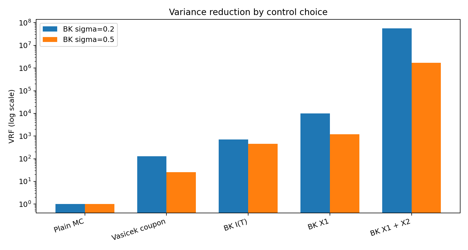
Figure 4. 통제변량별 VRF 비교. 큰 값과 작은 값이 함께 보이도록 로그 축을 사용했다.

Task 10 해석. 이번 계산에서는 BK의 쿠폰 가중 적분 금리 기반 통제변량이 더 높은 VRF를 보였다. 이는 할인계수의 Taylor 근사와 연결되지만, 이 결과가 모든 파라미터에서 성립하는 것은 아니다.

Part D Validation

모멘트의 기본 관계, 독립 표본의 통제변량 평균, σ=0에서의 결정론적 할인 가격 등을 검사한다. 허용오차와 검출 한계를 정리한 테스트 기록표는 제출 전 보완한다.

Python Implementation (Notebook 셀 41)

# Part D validation

for sigma in D_SIGMAS:

    Y, I = d_simulate_bk(
        d_z_pricing, sigma
    )

    controls = d_make_controls(I)
    mu = d_control_expectations(sigma)

    # Test 1: Finite, positive bond payoffs
    assert np.all(np.isfinite(Y))
    assert np.all(Y > 0)

    # Test 2: Moment consistency
    mean_I, mean_I2 = d_integrated_rate_moments(
        sigma
    )

    assert np.all(
        mean_I2 >= mean_I**2 - 1e-12
    )

    # Test 3: Control expectations versus MC means
    for name in ["IT", "IT2", "X1", "X2"]:
        X = controls[name]

        se_mean = np.std(
            X, ddof=1
        ) / np.sqrt(D_N)

        difference = abs(
            np.mean(X) - mu[name]
        )

        assert difference < 4 * se_mean, (
            f"Control expectation check failed: "
            f"sigma={sigma}, control={name}"
        )

    # Test 4: CV outputs are finite
    for name, result in d_task9_results[sigma].items():

        assert np.isfinite(result["price"])
        assert np.isfinite(result["se"])
        assert np.all(np.isfinite(result["nu"]))
        assert np.isfinite(result["vrf"])

        assert result["se"] > 0
        assert result["vrf"] > 0

    print(f"BK sigma={sigma}: validation passed")


# Test 5: Deterministic zero-volatility case
z_test = d_generate_normals(
    n=100,
    dt=D_DT,
    seed=9876
)

Y_zero, I_zero = d_simulate_bk(
    z_test, sigma=0.0
)

mu_zero = d_control_expectations(sigma=0.0)
controls_zero = d_make_controls(I_zero)

years = np.arange(1, D_T + 1)

expected_bond_price = np.sum(
    D_CASHFLOWS * np.exp(-D_R0 * years)
)

assert np.allclose(
    Y_zero,
    expected_bond_price,
    atol=1e-12
)

for name in ["IT", "IT2", "X1", "X2"]:
    assert np.allclose(
        controls_zero[name],
        mu_zero[name],
        atol=1e-12
    )

print("Zero-volatility validation passed.")
print("All Part D validation tests passed.")

저장된 실행 결과

BK sigma=0.2: validation passed
BK sigma=0.5: validation passed
Zero-volatility validation passed.
All Part D validation tests passed.

Part D 정리

BK 적분 금리만으로 통제변량을 구성하고 네 가지 조합의 SE와 VRF를 비교했다. 분산을 줄이는 것과 기대값이 정확한 것은 별개의 검증 대상임을 확인했다.

Part E: Testing the Known Expectations & Summary

통제변량의 기대값을 검증하고 이산화 및 기대값 오류가 CV 추정량에 미치는 영향을 실험한다. 마지막으로 전체 추정량을 같은 조건에서 비교한다.

Task 11. 통제변량 기대값 독립 검증

Part C·D에서 사용한 통제변량 기대값과 독립 Monte Carlo 표본평균을 비교한다. 두 값의 차이를 표본평균의 SE로 나눈 Z-score를 출력하고

Z

≤4를 통계적 허용 기준으로 사용한다. 현재 셀은 Part C 기본 파라미터만 검증하므로 다른 선택값은 추가 검증이 필요하다.

Python Implementation (Notebook 셀 44)

import numpy as np
import matplotlib.pyplot as plt
import time

# Part E simulation settings
E_SIGMAS = (0.2, 0.5)
E_DT = 1 / 52
E_N_TEST = 30000
E_SEED = 314159

E_ALPHA = 0.8
E_BETA = 0.03
E_ETA = 0.01

# Independent validation sample
z_test = d_generate_normals(
    E_N_TEST, E_DT, E_SEED
)

# Vasicek control expectations
mu_vas_z, mu_vas_c = d_vasicek_expectations(
    E_ALPHA, E_BETA, E_ETA, E_DT
)

# Same independent Gaussian increments
Xz, Xc = d_simulate_vasicek_controls(
    z_test, E_ALPHA, E_BETA, E_ETA, E_DT
)


def e_expectation_check(name, values, expected_mu):
    mean_mc = np.mean(values)
    se_mc = np.std(values, ddof=1) / np.sqrt(len(values))

    difference = mean_mc - expected_mu
    z_score = difference / se_mc

    passed = abs(z_score) <= 4

    return {
        "control": name,
        "expected": float(expected_mu),
        "mc_mean": float(mean_mc),
        "se": float(se_mc),
        "difference": float(difference),
        "z_score": float(z_score),
        "passed": bool(passed)
    }


e_task11_results = []

# Part C controls
e_task11_results.append(
    e_expectation_check(
        "Vasicek ZCB", Xz, mu_vas_z
    )
)

e_task11_results.append(
    e_expectation_check(
        "Vasicek coupon", Xc, mu_vas_c
    )
)

# Part D controls, for both BK volatility values
for sigma in E_SIGMAS:
    Y_test, I_test = d_simulate_bk(
        z_test, sigma, E_DT
    )

    controls = d_make_controls(I_test)
    expectations = d_control_expectations(sigma, E_DT)

    for name in ["IT", "IT2", "X1", "X2"]:
        result = e_expectation_check(
            f"BK sigma={sigma}, {name}",
            controls[name],
            expectations[name]
        )
        e_task11_results.append(result)


# Print validation table
print("=== Task 11: Control Expectation Validation ===")
print(
    f"{'Control':27s} {'Expected':>11s} "
    f"{'MC mean':>11s} {'Z-score':>10s} {'Pass':>6s}"
)

for r in e_task11_results:
    print(
        f"{r['control']:27s} "
        f"{r['expected']:11.7f} "
        f"{r['mc_mean']:11.7f} "
        f"{r['z_score']:10.3f} "
        f"{str(r['passed']):>6s}"
    )

assert all(r["passed"] for r in e_task11_results)

print("\nAll Task 11 expectation checks passed.")

저장된 실행 결과

=== Task 11: Control Expectation Validation ===
Control                        Expected     MC mean    Z-score   Pass
Vasicek ZCB                   0.8609221   0.8610819      1.454   True
Vasicek coupon                1.0438936   1.0440688      1.428   True
BK sigma=0.2, IT              0.1516649   0.1515368     -1.648   True
BK sigma=0.2, IT2             0.0231869   0.0231450     -1.749   True
BK sigma=0.2, X1              0.1698482   0.1697081     -1.621   True
BK sigma=0.2, X2              0.0252263   0.0251813     -1.733   True
BK sigma=0.5, IT              0.1607332   0.1603438     -1.847   True
BK sigma=0.5, IT2             0.0271900   0.0270429     -1.967   True
BK sigma=0.5, X1              0.1799125   0.1794867     -1.819   True
BK sigma=0.5, X2              0.0295760   0.0294177     -1.951   True

All Task 11 expectation checks passed.

Task 11 해석. 현재 확인한 기대값은 독립 MC의 4 SE 허용범위 안에 있었다. 다만 검정력이 유한하므로 통과했다고 해서 모든 미세한 오류가 배제되는 것은 아니다.

Task 12. 이산화가 통제변량 기대값에 미치는 영향

Δt=1/52와 1/252에서 통제변량 기대값을 비교하고 Vasicek에서는 사다리꼴과 왼쪽 직사각형 적분 결과도 비교한다. 서로 다른 방식으로 구한 기대값을 섞어 쓰면 생기는 CV 가격 이동을 SE 단위로 평가한다.

Python Implementation (Notebook 셀 47)

# Task 12: time-step effects

E_STEPS = (1 / 52, 1 / 252)

def e_continuous_vasicek_zcb(t, alpha, beta, eta, r0):
    B = -np.expm1(-alpha * t) / alpha
    A = (
        (beta - eta**2 / (2 * alpha**2)) * (B - t)
        - eta**2 * B**2 / (4 * alpha)
    )
    return np.exp(A - B * r0)


vas_cont_zcb = e_continuous_vasicek_zcb(
    D_T, E_ALPHA, E_BETA, E_ETA, D_R0
)

vas_cont_coupon = sum(
    D_CASHFLOWS[year - 1]
    * e_continuous_vasicek_zcb(
        year, E_ALPHA, E_BETA, E_ETA, D_R0
    )
    for year in range(1, D_T + 1)
)

e_task12_expectations = {}

print("=== Vasicek: discrete vs continuous ===")

for dt in E_STEPS:
    mu_z, mu_c = d_vasicek_expectations(
        E_ALPHA, E_BETA, E_ETA, dt
    )

    e_task12_expectations[("Vasicek", dt)] = (mu_z, mu_c)

    print(f"\ndt = {dt:.8f}")
    print(f"ZCB discrete:    {mu_z:.10f}")
    print(f"ZCB continuous:  {vas_cont_zcb:.10f}")
    print(f"ZCB difference:  {mu_z - vas_cont_zcb:+.10f}")
    print(f"Coupon discrete:   {mu_c:.10f}")
    print(f"Coupon continuous: {vas_cont_coupon:.10f}")
    print(f"Coupon difference: {mu_c - vas_cont_coupon:+.10f}")


print("\n=== BK: discrete control expectations ===")

for sigma in E_SIGMAS:
    print(f"\nBK sigma = {sigma}")

    for dt in E_STEPS:
        mu = d_control_expectations(sigma, dt)
        e_task12_expectations[(sigma, dt)] = mu

        print(f"dt={dt:.8f}: {mu}")

    coarse = e_task12_expectations[(sigma, E_STEPS[0])]
    fine = e_task12_expectations[(sigma, E_STEPS[1])]

    print("Differences (coarse - fine):")
    for name in ["IT", "IT2", "X1", "X2"]:
        print(f"{name}: {coarse[name] - fine[name]:+.10f}")

저장된 실행 결과

=== Vasicek: discrete vs continuous ===

dt = 0.01923077
ZCB discrete:    0.8609220553
ZCB continuous:  0.8609212015
ZCB difference:  +0.0000008538
Coupon discrete:   1.0438936455
Coupon continuous: 1.0438926820
Coupon difference: +0.0000009634

dt = 0.00396825
ZCB discrete:    0.8609213775
ZCB continuous:  0.8609212015
ZCB difference:  +0.0000001760
Coupon discrete:   1.0438928806
Coupon continuous: 1.0438926820
Coupon difference: +0.0000001986

=== BK: discrete control expectations ===

BK sigma = 0.2
dt=0.01923077: {'IT': 0.1516649462365563, 'IT2': 0.023186855000636046, 'X1': 0.16984816437304046, 'X2': 0.025226337976935968}
dt=0.00396825: {'IT': 0.15165327717174187, 'IT2': 0.02318269486844777, 'X1': 0.16983512578044205, 'X2': 0.025221793731939134}
Differences (coarse - fine):
IT: +0.0000116691
IT2: +0.0000041601
X1: +0.0000130386
X2: +0.0000045442

BK sigma = 0.5
dt=0.01923077: {'IT': 0.16073316165592397, 'IT2': 0.027189996095222484, 'X1': 0.1799124735617631, 'X2': 0.029575994136731204}
dt=0.00396825: {'IT': 0.16065572462433808, 'IT2': 0.02715914601134587, 'X1': 0.17982597968038702, 'X2': 0.029542299413942}
Differences (coarse - fine):
IT: +0.0000774370
IT2: +0.0000308501
X1: +0.0000864939
X2: +0.0000336947

Python Implementation (Notebook 셀 48)

def e_vasicek_expectations_with_rule(
    alpha, beta, eta, dt, rule="trapezoid"
):
    m = round(D_T / dt)
    steps_per_year = m // D_T

    mean = np.array([D_R0, 0.0])
    cov = np.zeros((2, 2))

    a = 1 - alpha * dt
    b = alpha * beta * dt
    q = eta * np.sqrt(dt)

    if rule == "trapezoid":
        w_old = dt * (1 + a) / 2
        w_noise = dt * q / 2
        w_shift = dt * b / 2
    elif rule == "left":
        w_old = dt
        w_noise = 0.0
        w_shift = 0.0
    else:
        raise ValueError("Unknown integration rule")

    A = np.array([
        [a, 0.0],
        [w_old, 1.0]
    ])

    shift = np.array([b, w_shift])
    noise = np.array([q, w_noise])

    coupon_mu = 0.0

    for k in range(1, m + 1):
        mean = A @ mean + shift
        cov = A @ cov @ A.T + np.outer(noise, noise)

        if k % steps_per_year == 0:
            year_index = k // steps_per_year - 1

            expected_discount = np.exp(
                -mean[1] + 0.5 * cov[1, 1]
            )

            coupon_mu += (
                D_CASHFLOWS[year_index] * expected_discount
            )

    zcb_mu = np.exp(
        -mean[1] + 0.5 * cov[1, 1]
    )

    return zcb_mu, coupon_mu


for dt in E_STEPS:
    trap = e_vasicek_expectations_with_rule(
        E_ALPHA, E_BETA, E_ETA, dt, "trapezoid"
    )

    left = e_vasicek_expectations_with_rule(
        E_ALPHA, E_BETA, E_ETA, dt, "left"
    )

    print(f"\nTime step = {dt:.8f}")

    for name, trap_mu, left_mu in zip(
        ["ZCB", "Coupon"], trap, left
    ):
        print(
            f"{name}: trapezoid={trap_mu:.10f}, "
            f"left={left_mu:.10f}, "
            f"difference={left_mu - trap_mu:+.10f}"
        )

저장된 실행 결과

Time step = 0.01923077
ZCB: trapezoid=0.8609220553, left=0.8609214338, difference=-0.0000006215
Coupon: trapezoid=1.0438936455, left=1.0438929251, difference=-0.0000007204

Time step = 0.00396825
ZCB: trapezoid=0.8609213775, left=0.8609212490, difference=-0.0000001285
Coupon: trapezoid=1.0438928806, left=1.0438927316, difference=-0.0000001490

Python Implementation (Notebook 셀 49)

# Task 12: expectation mismatch relative to standard error

e_task12_bias_results = []

for sigma in E_SIGMAS:
    Y_pilot, I_pilot = d_simulate_bk(
        d_z_pilot, sigma, D_DT
    )

    Y_price, I_price = d_simulate_bk(
        d_z_pricing, sigma, D_DT
    )

    cp = d_make_controls(I_pilot)
    cf = d_make_controls(I_price)

    mu_correct = d_control_expectations(sigma, D_DT)
    mu_fine = d_control_expectations(sigma, 1 / 252)

    for control_name, keys in {
        "I(T)": ["IT"],
        "I(T), I(T)^2": ["IT", "IT2"],
        "X1": ["X1"],
        "X1, X2": ["X1", "X2"]
    }.items():

        xp = np.column_stack([cp[k] for k in keys])
        xf = np.column_stack([cf[k] for k in keys])

        correct_vector = np.array([mu_correct[k] for k in keys])
        wrong_vector = np.array([mu_fine[k] for k in keys])

        result = d_fit_cv(
            Y_pilot, xp, Y_price, xf, correct_vector
        )

        shift = float(
            result["nu"] @ (wrong_vector - correct_vector)
        )

        ratio = abs(shift) / result["se"]

        e_task12_bias_results.append(
            (sigma, control_name, shift, ratio)
        )


print("=== Task 12: Expectation mismatch ===")
print("Mismatch: fine-grid mu used for coarse-grid controls")

for sigma, name, shift, ratio in e_task12_bias_results:
    print(
        f"sigma={sigma}, {name:14s}: "
        f"price shift={shift:+.9f}, "
        f"|shift|/SE={ratio:.3f}"
    )


# Repeat for both Vasicek controls
Xzp, Xcp = d_simulate_vasicek_controls(d_z_pilot)
Xzf, Xcf = d_simulate_vasicek_controls(d_z_pricing)

mu_vas_coarse = d_vasicek_expectations(
    E_ALPHA, E_BETA, E_ETA, D_DT
)
mu_vas_fine = d_vasicek_expectations(
    E_ALPHA, E_BETA, E_ETA, 1 / 252
)

for sigma in E_SIGMAS:
    Yp, _ = d_simulate_bk(d_z_pilot, sigma)
    Yf, _ = d_simulate_bk(d_z_pricing, sigma)

    for name, xp, xf, correct_mu, wrong_mu in zip(
        ["Vasicek ZCB", "Vasicek coupon"],
        [Xzp, Xcp],
        [Xzf, Xcf],
        mu_vas_coarse,
        mu_vas_fine
    ):
        result = d_fit_cv(
            Yp, xp, Yf, xf, [correct_mu]
        )

        shift = float(result["nu"][0] * (wrong_mu - correct_mu))

        print(
            f"sigma={sigma}, {name}: "
            f"price shift={shift:+.9f}, "
            f"|shift|/SE={abs(shift)/result['se']:.3f}"
        )

저장된 실행 결과

=== Task 12: Expectation mismatch ===
Mismatch: fine-grid mu used for coarse-grid controls
sigma=0.2, I(T)          : price shift=+0.000011125, |shift|/SE=3.225
sigma=0.2, I(T), I(T)^2  : price shift=+0.000010857, |shift|/SE=3.262
sigma=0.2, X1            : price shift=+0.000011220, |shift|/SE=12.123
sigma=0.2, X1, X2        : price shift=+0.000010953, |shift|/SE=899.334
sigma=0.5, I(T)          : price shift=+0.000072221, |shift|/SE=6.310
sigma=0.5, I(T), I(T)^2  : price shift=+0.000070604, |shift|/SE=7.919
sigma=0.5, X1            : price shift=+0.000072859, |shift|/SE=10.265
sigma=0.5, X1, X2        : price shift=+0.000071264, |shift|/SE=382.602
sigma=0.2, Vasicek ZCB: price shift=-0.000000456, |shift|/SE=0.052
sigma=0.2, Vasicek coupon: price shift=-0.000000463, |shift|/SE=0.057
sigma=0.5, Vasicek ZCB: price shift=-0.000001195, |shift|/SE=0.024
sigma=0.5, Vasicek coupon: price shift=-0.000001212, |shift|/SE=0.025

Task 12 해석. BK [X₁,X₂] 통제변량에서는 작은 기대값 차이도 CV 표준오차보다 수백 배 크게 나타났다. 이는 분산 감소에 성공했더라도 기대값 불일치를 방치하면 편향이 심각해질 수 있음을 보여준다. BK에서 적분 규칙 자체를 바꾼 비교는 추가할 예정이다.

Task 13. 의도적으로 틀린 기대값 사용

BK X₁의 기대값에 δ=0.005를 더해 CV 가격, SE와 95% 신뢰구간 포함률이 어떻게 달라지는지 비교한다. 반복 횟수 80회는 과제 지시값이 아니라 실험을 위해 선택한 값이며, 기준 가격도 큰 독립 MC 표본으로 얻은 수치적 추정값이다.

Python Implementation (Notebook 셀 52)

E_DELTA = 0.005

e_task13_results = {}

for sigma in E_SIGMAS:
    # BK pilot and pricing paths
    Yp, Ip = d_simulate_bk(d_z_pilot, sigma)
    Y, I = d_simulate_bk(d_z_pricing, sigma)

    # Use the BK control X1 for this illustration
    Xp = d_make_controls(Ip)["X1"]
    X = d_make_controls(I)["X1"]

    correct_mu = d_control_expectations(sigma)["X1"]
    incorrect_mu = correct_mu + E_DELTA

    correct = d_fit_cv(
        Yp, Xp, Y, X, [correct_mu]
    )

    incorrect = d_fit_cv(
        Yp, Xp, Y, X, [incorrect_mu]
    )

    e_task13_results[sigma] = {
        "correct": correct,
        "incorrect": incorrect
    }

    actual_shift = incorrect["price"] - correct["price"]
    predicted_shift = correct["nu"][0] * E_DELTA

    print(f"\n=== BK sigma = {sigma} ===")
    print(f"Correct CV price:   {correct['price']:.8f}")
    print(f"Incorrect CV price: {incorrect['price']:.8f}")
    print(f"Correct SE:         {correct['se']:.8f}")
    print(f"Incorrect SE:       {incorrect['se']:.8f}")
    print(f"Price shift:        {actual_shift:+.8f}")
    print(f"Predicted shift:    {predicted_shift:+.8f}")

    # Changing only mu must not change the SE
    assert np.isclose(
        correct["se"],
        incorrect["se"],
        atol=1e-12,
        rtol=1e-12
    )

    assert np.isclose(
        actual_shift,
        predicted_shift,
        atol=1e-12
    )

print("\nIncorrect-expectation shift tests passed.")

저장된 실행 결과

=== BK sigma = 0.2 ===
Correct CV price:   1.04215044
Incorrect CV price: 1.03784782
Correct SE:         0.00000093
Incorrect SE:       0.00000093
Price shift:        -0.00430262
Predicted shift:    -0.00430262

=== BK sigma = 0.5 ===
Correct CV price:   1.03405042
Incorrect CV price: 1.02983861
Correct SE:         0.00000710
Incorrect SE:       0.00000710
Price shift:        -0.00421180
Predicted shift:    -0.00421180

Incorrect-expectation shift tests passed.

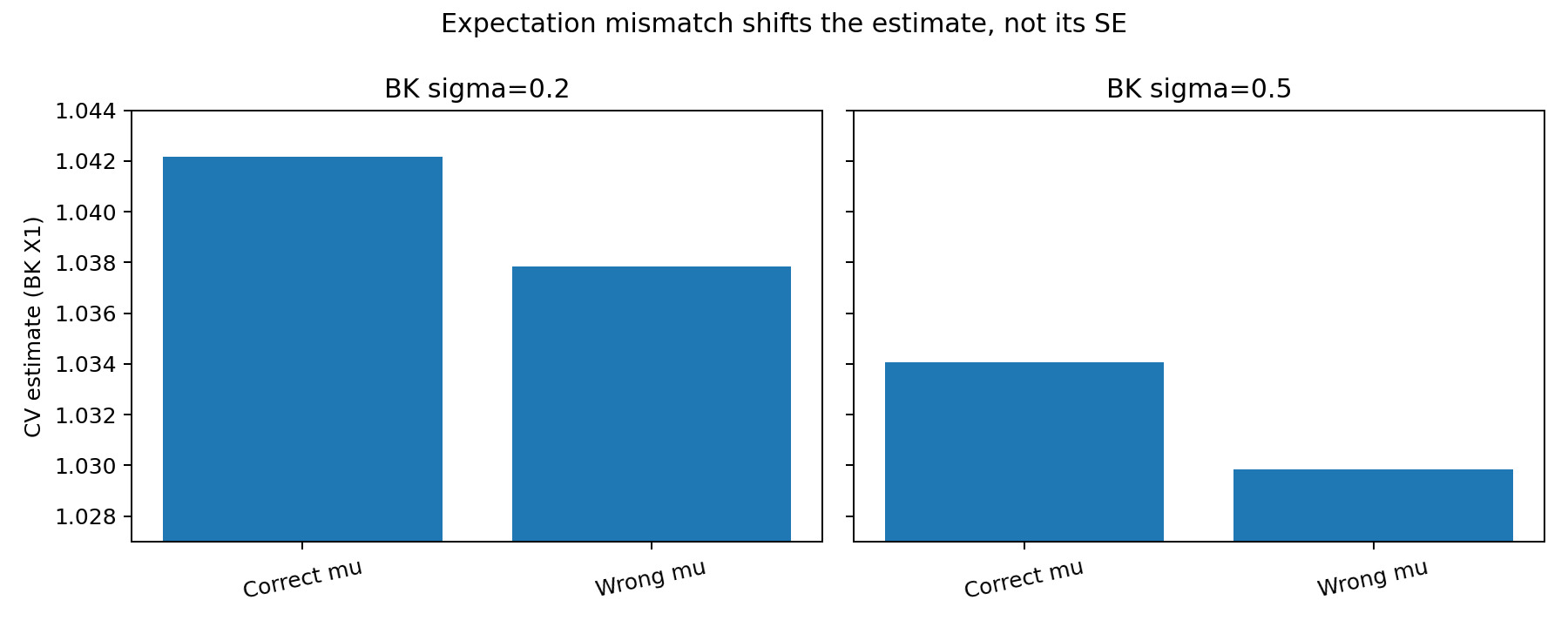
Figure 5. 통제변량 기대값의 오류가 CV 가격을 이동시키지만 SE를 바꾸지는 않는 사례.

Python Implementation (Notebook 셀 53)

# Task 13: Confidence interval coverage experiment
# Uses the Part D X1 control and independent simulations.

E_REPETITIONS = 80
E_N_COVERAGE = 2000
E_N_REFERENCE = 120000

e_coverage_results = {}

for sigma in E_SIGMAS:
    mu = d_control_expectations(sigma)["X1"]

    # Estimate nu using independent pilot paths
    Yp, Ip = d_simulate_bk(d_z_pilot, sigma)
    Xp = d_make_controls(Ip)["X1"]

    nu = np.cov(Xp, Yp, ddof=1)[0, 1] / np.var(
        Xp, ddof=1
    )

    # Independent, larger reference calculation.
    # Process in batches to avoid excessive memory use.
    reference_cv_sum = 0.0
    reference_cv_sumsq = 0.0
    processed = 0

    batch_size = 10000

    for batch in range(E_N_REFERENCE // batch_size):
        zb = d_generate_normals(
            batch_size,
            D_DT,
            700000 + 1000 * int(sigma * 10) + batch
        )

        Yb, Ib = d_simulate_bk(zb, sigma)
        Xb = d_make_controls(Ib)["X1"]

        cvb = Yb - nu * (Xb - mu)

        reference_cv_sum += np.sum(cvb)
        reference_cv_sumsq += np.sum(cvb**2)
        processed += len(cvb)

    reference_price = reference_cv_sum / processed

    reference_var = (
        reference_cv_sumsq
        - processed * reference_price**2
    ) / (processed - 1)

    reference_se = np.sqrt(
        max(reference_var, 0) / processed
    )

    covered_correct = 0
    covered_incorrect = 0

    widths_correct = []
    widths_incorrect = []

    for rep in range(E_REPETITIONS):
        z = d_generate_normals(
            E_N_COVERAGE,
            D_DT,
            900000 + 10000 * int(sigma * 10) + rep
        )

        Y, I = d_simulate_bk(z, sigma)
        X = d_make_controls(I)["X1"]

        cv_correct = Y - nu * (X - mu)
        cv_incorrect = Y - nu * (X - (mu + E_DELTA))

        price_correct = np.mean(cv_correct)
        price_incorrect = np.mean(cv_incorrect)

        se_correct = np.std(
            cv_correct, ddof=1
        ) / np.sqrt(E_N_COVERAGE)

        se_incorrect = np.std(
            cv_incorrect, ddof=1
        ) / np.sqrt(E_N_COVERAGE)

        # Approximate 95% normal confidence intervals
        lower_correct = price_correct - 1.96 * se_correct
        upper_correct = price_correct + 1.96 * se_correct

        lower_incorrect = price_incorrect - 1.96 * se_incorrect
        upper_incorrect = price_incorrect + 1.96 * se_incorrect

        covered_correct += (
            lower_correct <= reference_price <= upper_correct
        )

        covered_incorrect += (
            lower_incorrect <= reference_price <= upper_incorrect
        )

        widths_correct.append(upper_correct - lower_correct)
        widths_incorrect.append(upper_incorrect - lower_incorrect)

    e_coverage_results[sigma] = {
        "reference": reference_price,
        "reference_se": reference_se,
        "correct_coverage": covered_correct / E_REPETITIONS,
        "incorrect_coverage": covered_incorrect / E_REPETITIONS,
        "correct_width": np.mean(widths_correct),
        "incorrect_width": np.mean(widths_incorrect),
        "nu": nu
    }

    print(f"\n=== BK sigma = {sigma} ===")
    print(f"Reference price: {reference_price:.8f}")
    print(f"Reference SE:    {reference_se:.8f}")
    print(
        f"Correct mu coverage: "
        f"{covered_correct / E_REPETITIONS:.1%}"
    )
    print(
        f"Incorrect mu coverage: "
        f"{covered_incorrect / E_REPETITIONS:.1%}"
    )
    print(
        f"Correct mean CI width: "
        f"{np.mean(widths_correct):.8f}"
    )
    print(
        f"Incorrect mean CI width: "
        f"{np.mean(widths_incorrect):.8f}"
    )

저장된 실행 결과

=== BK sigma = 0.2 ===
Reference price: 1.04215049
Reference SE:    0.00000037
Correct mu coverage: 92.5%
Incorrect mu coverage: 0.0%
Correct mean CI width: 0.00001127
Incorrect mean CI width: 0.00001127

=== BK sigma = 0.5 ===
Reference price: 1.03404736
Reference SE:    0.00000280
Correct mu coverage: 97.5%
Incorrect mu coverage: 0.0%
Correct mean CI width: 0.00008549
Incorrect mean CI width: 0.00008549

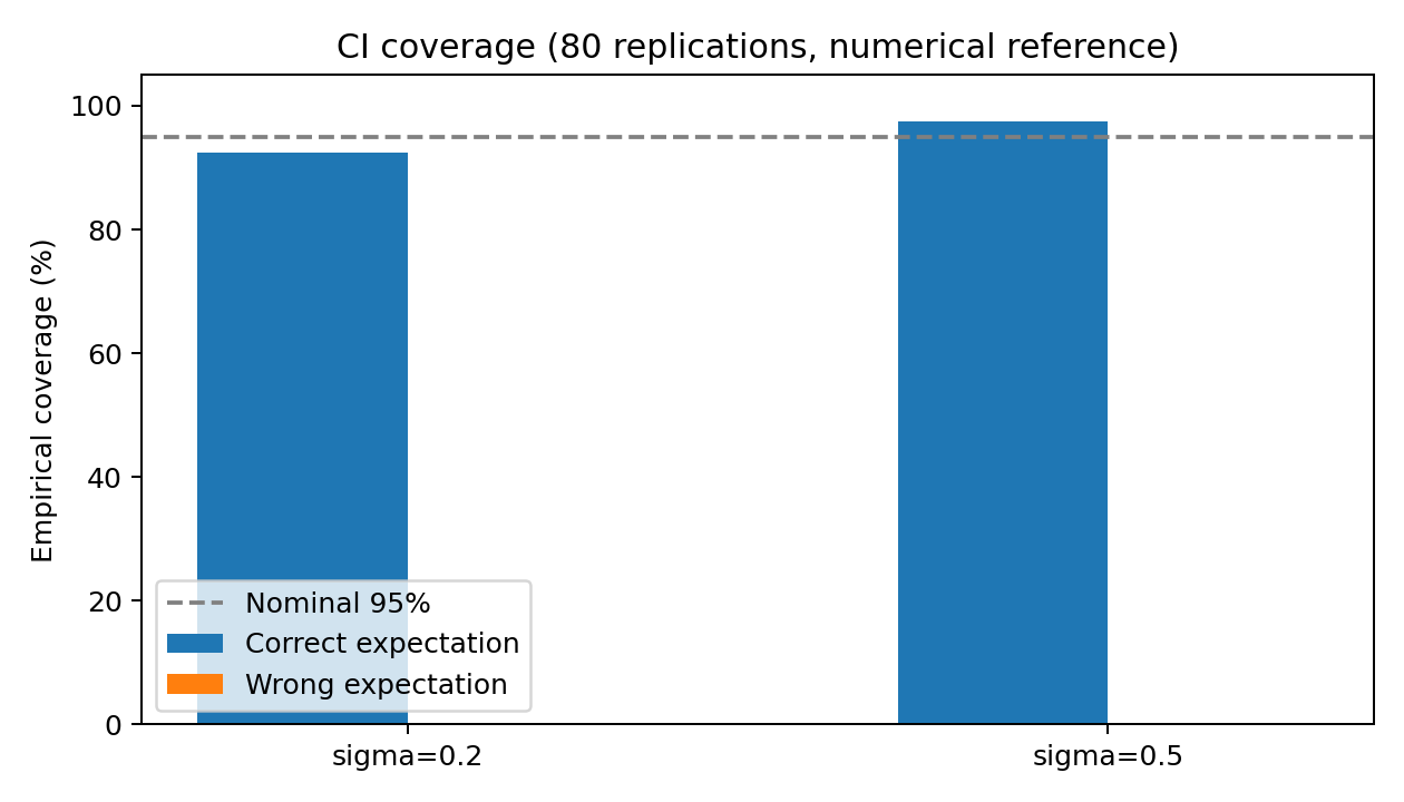
Figure 6. 80회 반복으로 확인한 95% 신뢰구간의 경험적 포함률. 기준 가격도 수치 추정값이다.

Task 14. 전체 추정량 비교

두 BK 변동성에서 Plain MC, Vasicek 통제변량(기본값·근사값·격자값), BK 경로 기반 통제변량의 가격·SE·VRF·실행 시간을 정리한다. 실행 시간은 컴퓨터 환경과 구현 방식에 의존하므로 상대적 비교 지표로 해석한다.

Python Implementation (Notebook 셀 55)

import time
import numpy as np

E_SUMMARY = []

# Previously generated independent samples
# d_z_pilot: coefficient estimation
# d_z_pricing: final pricing

def e_add_summary(sigma, method, result, elapsed):
    E_SUMMARY.append({
        "sigma": sigma,
        "method": method,
        "price": result["price"],
        "se": result["se"],
        "vrf": result["vrf"],
        "seconds": elapsed
    })


for sigma in E_SIGMAS:

    # Plain Monte Carlo
    start = time.perf_counter()

    Yp, Ip = d_simulate_bk(d_z_pilot, sigma)
    Y, I = d_simulate_bk(d_z_pricing, sigma)

    elapsed = time.perf_counter() - start

    plain_price = float(np.mean(Y))
    plain_se = float(
        np.std(Y, ddof=1) / np.sqrt(len(Y))
    )

    e_add_summary(
        sigma,
        "Plain MC",
        {
            "price": plain_price,
            "se": plain_se,
            "vrf": 1.0
        },
        elapsed
    )

    # Vasicek parameter configurations
    vasicek_choices = {
        "Baseline": (0.8, 0.03, 0.01),
        "Matched": (
            D_KAPPA,
            np.exp(D_THETA),
            sigma * np.exp(D_THETA)
        )
    }

    # Optionally include Part C grid-search choices
    if all(
        name in globals()
        for name in ["grid_results", "alpha_grid", "eta_grid"]
    ):
        for index, label in [
            (0, "Grid ZCB"),
            (1, "Grid Coupon")
        ]:
            vrf_grid = grid_results[sigma][index]

            iy, ix = np.unravel_index(
                np.argmax(vrf_grid),
                vrf_grid.shape
            )

            vasicek_choices[label] = (
                float(alpha_grid[ix]),
                0.03,
                float(eta_grid[iy])
            )

    # Part C: Vasicek controls
    for choice_name, params in vasicek_choices.items():
        alpha, beta, eta = params

        for control_name in ["ZCB", "Coupon"]:

            # A grid optimum is specific to its own control
            if choice_name == "Grid ZCB" and control_name != "ZCB":
                continue

            if choice_name == "Grid Coupon" and control_name != "Coupon":
                continue

            start = time.perf_counter()

            Xzp, Xcp = d_simulate_vasicek_controls(
                d_z_pilot, alpha, beta, eta
            )

            Xz, Xc = d_simulate_vasicek_controls(
                d_z_pricing, alpha, beta, eta
            )

            mu_z, mu_c = d_vasicek_expectations(
                alpha, beta, eta
            )

            if control_name == "ZCB":
                xp, xf, mu = Xzp, Xz, mu_z
            else:
                xp, xf, mu = Xcp, Xc, mu_c

            # Include target BK simulation cost
            Yp_local, _ = d_simulate_bk(
                d_z_pilot, sigma
            )
            Y_local, _ = d_simulate_bk(
                d_z_pricing, sigma
            )

            result = d_fit_cv(
                Yp_local, xp, Y_local, xf, [mu]
            )

            elapsed = time.perf_counter() - start

            e_add_summary(
                sigma,
                f"Vasicek {control_name} ({choice_name})",
                result,
                elapsed
            )

    # Part D: BK path-based controls
    configurations = {
        "I(T)": ["IT"],
        "I(T), I(T)^2": ["IT", "IT2"],
        "X1": ["X1"],
        "X1, X2": ["X1", "X2"]
    }

    for control_name, keys in configurations.items():
        start = time.perf_counter()

        Yp_local, Ip_local = d_simulate_bk(
            d_z_pilot, sigma
        )
        Y_local, I_local = d_simulate_bk(
            d_z_pricing, sigma
        )

        cp = d_make_controls(Ip_local)
        cf = d_make_controls(I_local)

        mu_all = d_control_expectations(sigma)

        xp = np.column_stack([cp[k] for k in keys])
        xf = np.column_stack([cf[k] for k in keys])
        mu = np.array([mu_all[k] for k in keys])

        result = d_fit_cv(
            Yp_local, xp, Y_local, xf, mu
        )

        elapsed = time.perf_counter() - start

        e_add_summary(
            sigma,
            f"BK {control_name}",
            result,
            elapsed
        )


# Print final comparison table
print("=== Task 14: Final Estimator Comparison ===")

header = (
    f"{'Sigma':>5} {'Method':36s} "
    f"{'Price':>12} {'SE':>12} "
    f"{'VRF':>9} {'Time(s)':>9}"
)
print(header)
print("-" * len(header))

for r in E_SUMMARY:
    print(
        f"{r['sigma']:5.1f} "
        f"{r['method']:36s} "
        f"{r['price']:12.8f} "
        f"{r['se']:12.8f} "
        f"{r['vrf']:9.2f} "
        f"{r['seconds']:9.4f}"
    )

# Identify highest-VRF method for each BK volatility
for sigma in E_SIGMAS:
    candidates = [
        r for r in E_SUMMARY
        if r["sigma"] == sigma
    ]

    best = max(candidates, key=lambda r: r["vrf"])

    print(f"\nBest VRF for BK sigma={sigma}:")
    print(f"Method: {best['method']}")
    print(f"VRF:    {best['vrf']:.2f}")
    print(f"SE:     {best['se']:.8f}")

저장된 실행 결과

=== Task 14: Final Estimator Comparison ===
Sigma Method                                      Price           SE       VRF   Time(s)
----------------------------------------------------------------------------------------
  0.2 Plain MC                               1.04212403   0.00009197      1.00    0.1810
  0.2 Vasicek ZCB (Baseline)                 1.04216099   0.00000884    108.36    0.2332
  0.2 Vasicek Coupon (Baseline)              1.04215894   0.00000816    127.16    0.2323
  0.2 Vasicek ZCB (Matched)                  1.04216098   0.00000837    120.78    0.2319
  0.2 Vasicek Coupon (Matched)               1.04215895   0.00000766    144.01    0.2283
  0.2 Vasicek ZCB (Grid ZCB)                 1.04215872   0.00000730    158.51    0.3134
  0.2 Vasicek Coupon (Grid Coupon)           1.04215954   0.00000721    162.75    0.3508
  0.2 BK I(T)                                1.04215152   0.00000345    710.86    0.2527
  0.2 BK I(T), I(T)^2                        1.04215154   0.00000333    763.39    0.1898
  0.2 BK X1                                  1.04215044   0.00000093   9873.68    0.2491
  0.2 BK X1, X2                              1.04215038   0.00000001 57026630.30    0.2835
  0.5 Plain MC                               1.03400908   0.00024446      1.00    0.1771
  0.5 Vasicek ZCB (Baseline)                 1.03410593   0.00004926     24.63    0.2261
  0.5 Vasicek Coupon (Baseline)              1.03410052   0.00004851     25.39    0.2250
  0.5 Vasicek ZCB (Matched)                  1.03410588   0.00005083     23.13    0.2276
  0.5 Vasicek Coupon (Matched)               1.03410040   0.00005007     23.84    0.2264
  0.5 Vasicek ZCB (Grid ZCB)                 1.03410006   0.00004620     28.00    0.2215
  0.5 Vasicek Coupon (Grid Coupon)           1.03410222   0.00004607     28.15    0.2246
  0.5 BK I(T)                                1.03404968   0.00001145    456.13    0.2611
  0.5 BK I(T), I(T)^2                        1.03404802   0.00000892    751.80    0.1808
  0.5 BK X1                                  1.03405042   0.00000710   1186.30    0.1917
  0.5 BK X1, X2                              1.03404842   0.00000019 1722574.84    0.1787

Best VRF for BK sigma=0.2:
Method: BK X1, X2
VRF:    57026630.30
SE:     0.00000001

Best VRF for BK sigma=0.5:
Method: BK X1, X2
VRF:    1722574.84
SE:     0.00000019

통제변량은 BK 쿠폰 채권 가격의 통계적 정밀도를 크게 개선할 수 있다. 그러나 VRF가 높더라도 기대값이 잘못되면 가격이 이동하고 SE에는 그 편향이 드러나지 않는다. 따라서 분산 감소 결과와 기대값 검증, 이산화 오차 분석을 함께 평가해야 한다. 최종적인 실무 선택은 VRF뿐 아니라 추가 계산 비용과 기대값의 신뢰성까지 고려할 예정이다.

---

검토하면서 수정할 사항

이 글과 Jupyter Notebook은 아래 사항을 함께 수정할 예정이다.

• Task 11: Part C에서 사용한 Baseline·Matched·Grid 파라미터까지 독립 기대값 검증 범위 확대
• Task 12: BK 통제변량에서 적분 규칙 변경의 영향 추가 비교
• Task 13: 신뢰구간 포함률 실험의 반복 수, 수치 기준 가격의 불확실성 명시
• Task 14: 실제 출력값에 근거한 최종 방법 선택 및 전체 실행 시간 확인
• Assessment Rules: 테스트 등록표(검증 대상·검출 가능/불가능 오류·허용오차 근거), AI 사용 선언 및 Restart & Run All 확인