Euler Schemes, Consistency and Convergence

Introduction

Lec-2_3_scheme.pdf의 1–4쪽을 중심으로 Forward/Backward Euler, Local Truncation Error, Consistency, Global Convergence 및 Leap-Frog의 불안정성을 공부한다. LAB_1.ipynb의 Python Exercise 1–3은 설명 직후에 배치했고, Lab Handout의 Forward/Backward Euler 문제도 함께 풀이했다.

8. Numerical Solutions of ODEs

실제 ODE는 정확한 해를 초등함수 형태로 나타내기 어려운 경우가 많다. 따라서 t₀, t₁, …, tₙ의 격자점에서 해를 근사한다.

8.1 Forward Euler Method

Forward Euler는 현재 위치에서의 기울기를 이용해 다음 지점을 예측하는 가장 기본적인 명시적 수치 스킴이다.

계산 과정은 다음과 같다.

1. 초기값 y₀과 시간 간격 h를 지정한다.
2. 현재 위치에서 기울기 f(tₙ,yₙ)를 계산한다.
3. yₙ₊₁ = yₙ + h·f(tₙ,yₙ)로 한 단계 진행한다.
4. 목표 시간까지 반복한다.

기울기를 현재 시점에서 한 번만 계산하므로 구현이 간단하다. 반면 오차가 비교적 크고 시간 간격에 따라 안정성 문제가 발생할 수 있다.

8.2 Lecture Example — Two Euler Steps

강의의 예제는 y'=t−y, y(0)=1, h=0.2이다.

• 첫 단계: f(0,1)=−1이므로 y₁=1+0.2(−1)=0.8.
• 두 번째 단계: f(0.2,0.8)=−0.6이므로 y₂=0.8+0.2(−0.6)=0.68.

이처럼 미분방정식의 우변을 매번 현재 근삿값에 대입한다는 점이 Euler의 핵심이다.

8.3 Local Truncation Error, Consistency, and Global Error

여기서 세 개념을 구분해야 한다.

• Local Truncation Error (LTE): 이전 단계에 정확한 값을 넣었다고 가정할 때 한 단계의 수치식이 만족하지 못하는 차이.
• Consistency: 시간 간격 h → 0일 때 적절히 정규화한 LTE가 0으로 수렴하는 성질.
• Global Error: 시작점부터 반복한 근삿값 yₙ과 정확한 값 y(tₙ) 사이의 차이.

여기서는 h로 나눈 정규화 LTE를 사용한다. 이 정의에 따르면 Forward Euler의 LTE는 보통 O(h)이고, 한 단계 업데이트 자체의 결함은 O(h²)이다. 두 표기가 혼용되므로 정의를 확인해야 한다.

8.4 Notebook Experiment 1 — Forward Euler LTE and Consistency

업로드한 LAB_1.ipynb의 첫 번째 실험에서는 y'=−y, 정확한 해 y(t)=e^(−t)를 사용한다. 고정된 지점 t=1에서 h를 변화시키며 정규화 LTE를 계산한다. 이 실험은 Lab-1.pdf의 Exercise 1과는 별개의 실험이다.

Taylor 전개를 적용하면 LTE의 선도항 크기는 e^(−1)·h/2이므로 h가 충분히 작아지면 로그-로그 그래프에서 기울기 약 1을 기대한다.

Python Implementation

import numpy as np
import matplotlib.pyplot as plt

# Exercise 1: Forward Euler LTE and Consistency

# Fixed evaluation point
x_n = 1.0

# Number of grid intervals
n_values = [10, 100, 1000, 10000]

# Lists to store results
h_values = []
lte_values = []

# Calculate LTE for different step sizes
for n in n_values:
    h = 1 / n
    x_prev = x_n - h

    # Exact solution y(x) = exp(-x)
    y_n = np.exp(-x_n)
    y_prev = np.exp(-x_prev)

    # Forward Euler LTE
    lte = (y_n - y_prev) / h + y_prev

    h_values.append(h)
    lte_values.append(abs(lte))

    print(f"n = {n:5d}, h = {h:.5f}, LTE = {lte:.10f}")

# Plot the results
plt.figure(figsize=(7, 5))
plt.loglog(h_values, lte_values, 'o-', label='LTE')
plt.loglog(h_values, np.exp(-x_n) * np.array(h_values) / 2,
           '--', label='Reference: exp(-1)*h/2')

plt.xlabel('Step size (h)')
plt.ylabel('Absolute LTE')
plt.title('Forward Euler: LTE and Consistency')
plt.legend()
plt.grid(True, which='both')
plt.tight_layout()
plt.show()

실행 결과

n =    10, h = 0.10000, LTE = 0.0196674740
n =   100, h = 0.01000, LTE = 0.0018517060
n =  1000, h = 0.00100, LTE = 0.0001840624
n = 10000, h = 0.00010, LTE = 0.0000183952

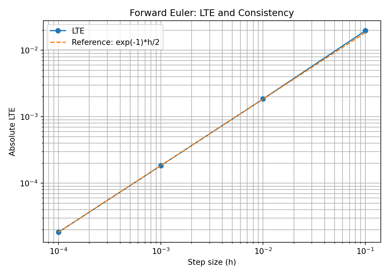
Figure 1. Forward Euler의 정규화 LTE와 이론적 기준선. 시간 간격이 작아질수록 LTE가 0에 가까워진다.

Results and Analysis. h=0.1일 때 LTE가 약 0.019667이었으나 h=0.0001에서 약 0.0000184로 감소했다. 수치 LTE가 기준선 e^(−1)·h/2에 점차 가까워지므로 이 예제에서 Forward Euler의 Consistency를 확인할 수 있다.

8.5 Notebook Experiment 2 — Forward Euler Global Convergence

두 번째 실험은 y'=−2y, y(0)=1이며 T=1에서 정확한 해 e^(−2)와 수치해를 비교한다.

Global Error를 여러 h에 대해 계산한 다음, ln(Error)와 ln(h)의 선형 회귀 기울기 p로 수렴 차수를 추정한다.

기울기가 약 1이면 오차가 h에 비례한다는 뜻이다.

Python Implementation

import numpy as np
import matplotlib.pyplot as plt

# Exercise 2: Forward Euler Convergence

# Initial condition and final time
y0 = 1.0
T = 1.0

# Exact solution: y(x) = exp(-2x)
exact_y = np.exp(-2 * T)

# Number of grid intervals
n_values = [10, 20, 40, 80, 160]

# Lists to store results
h_values = []
error_values = []

# Solve the IVP using Forward Euler
for n in n_values:
    h = T / n
    y = y0

    for i in range(n):
        y = y - 2 * h * y

    # Global error at T = 1
    error = abs(exact_y - y)

    h_values.append(h)
    error_values.append(error)

    print(f"n = {n:3d}, h = {h:.5f}, "
          f"y_n = {y:.10f}, Error = {error:.10f}")

# Estimate the empirical order of convergence
log_h = np.log(h_values)
log_error = np.log(error_values)

p, intercept = np.polyfit(log_h, log_error, 1)

print(f"\nEstimated convergence order p = {p:.6f}")

# Plot ln(Error) versus ln(h)
plt.figure(figsize=(7, 5))
plt.plot(log_h, log_error, 'o-', label='Global Error')
plt.plot(log_h, p * log_h + intercept,
         '--', label=f'Fitted line (p = {p:.4f})')

plt.xlabel('ln(h)')
plt.ylabel('ln(Error)')
plt.title('Forward Euler: Global Convergence')
plt.legend()
plt.grid(True)
plt.tight_layout()
plt.show()

실행 결과

n =  10, h = 0.10000, y_n = 0.1073741824, Error = 0.0279611008
n =  20, h = 0.05000, y_n = 0.1215766546, Error = 0.0137586286
n =  40, h = 0.02500, y_n = 0.1285121566, Error = 0.0068231267
n =  80, h = 0.01250, y_n = 0.1319378054, Error = 0.0033974778
n = 160, h = 0.00625, y_n = 0.1336400679, Error = 0.0016952153

Estimated convergence order p = 1.010556

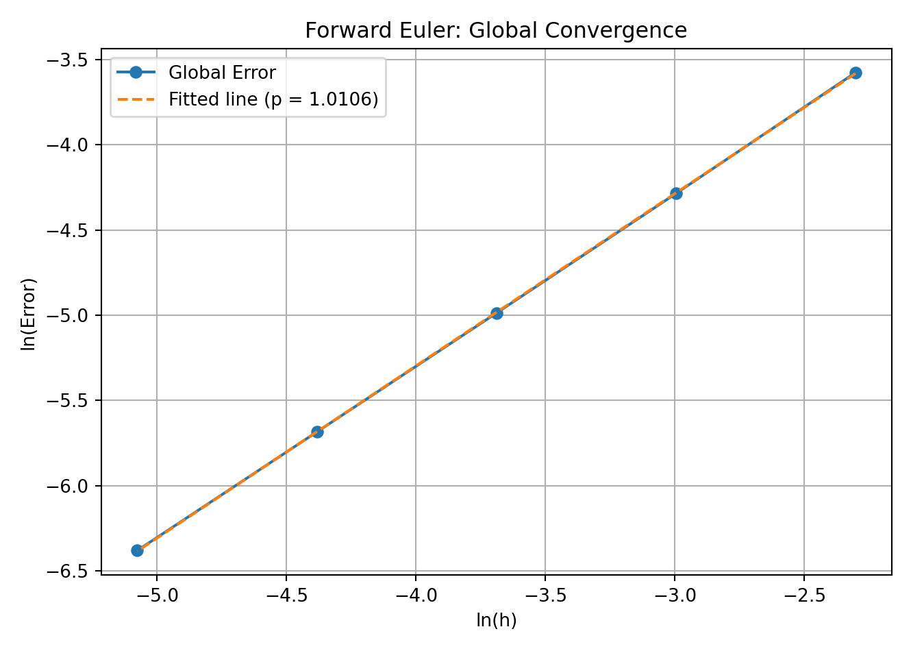
Figure 2. Forward Euler의 Global Error를 이용한 경험적 수렴차수 추정.

Results and Analysis. 시간 간격을 절반으로 줄이면 Global Error도 대략 절반으로 감소했다. 선형 회귀로 구한 수렴차수는 p ≈ 1.010556이므로 이 문제에서 Forward Euler의 1차 수렴(First-order Convergence)을 확인할 수 있다.

8.6 Stability and the Difference Between Consistency and Convergence

Consistency는 한 단계의 수치식이 미분방정식을 잘 근사하는지를 확인하는 조건이다. 반면 Stability는 수치 연산 중 생긴 작은 오차가 반복 계산을 거치며 어떻게 전파되는지를 다룬다.

특히 다단계 방법에서는 정확한 미분방정식에서 유래하지 않은 parasitic mode가 추가로 나타날 수 있다. 따라서 Consistency만 확인해서는 전체 알고리즘의 수렴성을 일반적으로 보장할 수 없다.

8.7 Notebook Experiment 3 — Leap-Frog and Long-Time Instability

세 번째 실험은 다음 ODE와 다단계 스킴을 사용한다.

Notebook에서는 두 초기 데이터를 y₀=1, y₁=1로 지정했다. 하지만 정확한 해의 첫 번째 다음 값은 y(h)=e^(−h)이므로 시작값 y₁=1에는 O(h)의 시작 오차가 있다. 이 때문에 고정 시간 T=1에서 관찰하는 수렴차수가 스킴 자체의 형식적 정확도와 다를 수 있다.

특성방정식을 세우면 다음과 같다.

한 근은 약 1−h로 감소하는 해를 따라가지만, 다른 근은 −1−h에 가까워 절댓값이 1보다 크다. 후자의 근이 불안정한 기생 모드를 생성한다. 고정된 T=1의 수치 오차가 감소하는 현상과 긴 시간에 진동이 증폭되는 현상은 모순이 아니다.

Python Implementation

import numpy as np
import matplotlib.pyplot as plt

# Exercise 3: Consistency Does Not Imply Convergence
# Method: Leap-Frog
# ODE: y' = -y, y(0) = 1
# Scheme: y[n+1] = y[n-1] - 2*h*y[n]

# Initial values and final time
y0 = 1.0
y1 = 1.0
T = 1.0

# Different grid sizes
n_values = [10, 20, 40, 80, 160]

# Exact solution at T = 1
exact_y = np.exp(-T)

h_values = []
numerical_values = []
error_values = []

# Apply the Leap-Frog scheme
for n in n_values:
    h = T / n

    y = np.zeros(n + 1)
    y[0] = y0
    y[1] = y1

    for i in range(1, n):
        y[i + 1] = y[i - 1] - 2 * h * y[i] 

    # Numerical solution and global error at T = 1
    numerical_y = y[-1]
    error = abs(exact_y - numerical_y)

    h_values.append(h)
    numerical_values.append(numerical_y)
    error_values.append(error)

    print(f"n = {n:3d}, h = {h:.5f}, "
          f"y(T) = {numerical_y:.10f}, "
          f"Error = {error:.10f}")


# Plot 1: Numerical vs Exact Solution at T = 1
plt.figure(figsize=(9, 5))

plt.plot(n_values, numerical_values, 'o-',
         label='Leap-Frog numerical solution')

plt.plot(n_values, [exact_y] * len(n_values), 'o-',
         label='Exact solution')

plt.xlabel('Grid Size (n)')
plt.ylabel('Solution at T = 1')
plt.title('Leap-Frog Method: Numerical vs Exact Solution')
plt.xticks(n_values)
plt.legend()
plt.grid(True, alpha=0.3)
plt.tight_layout()
plt.show()


# Plot 2: Global Error vs Step Size
plt.figure(figsize=(8, 5))

plt.loglog(h_values, error_values, 'o-',
           label='Global Error')

# Decreasing step size from left to right
plt.gca().invert_xaxis()

plt.xlabel('Step Size (h)')
plt.ylabel('Global Error at T = 1')
plt.title('Leap-Frog Method: Global Error')
plt.legend()
plt.grid(True, which='both', alpha=0.3)
plt.tight_layout()
plt.show()


# Plot 3: Long-Time Instability (Additional Analysis)
# Fixed step size h = 0.1 and extended time T = 20

h_long = 0.1
T_long = 20.0
n_long = int(T_long / h_long)

x_long = np.linspace(0, T_long, n_long + 1)
y_long = np.zeros(n_long + 1)

y_long[0] = 1.0
y_long[1] = 1.0

for i in range(1, n_long):
    y_long[i + 1] = y_long[i - 1] - 2 * h_long * y_long[i]

plt.figure(figsize=(9, 5))

plt.plot(x_long, y_long,
         label='Leap-Frog (h = 0.1)')

plt.plot(x_long, np.exp(-x_long), 'k--',
         linewidth=2, label='Exact Solution')

plt.xlabel('Time (t)')
plt.ylabel('y(t)')
plt.title('Leap-Frog Method: Long-Time Instability')
plt.legend()
plt.grid(True, alpha=0.3)
plt.tight_layout()
plt.show()

실행 결과

n =  10, h = 0.10000, y(T) = 0.2576276480, Error = 0.1102517932
n =  20, h = 0.05000, y(T) = 0.3108433549, Error = 0.0570360863
n =  40, h = 0.02500, y(T) = 0.3389179443, Error = 0.0289614969
n =  80, h = 0.01250, y(T) = 0.3532924543, Error = 0.0145869868
n = 160, h = 0.00625, y(T) = 0.3605599872, Error = 0.0073194539

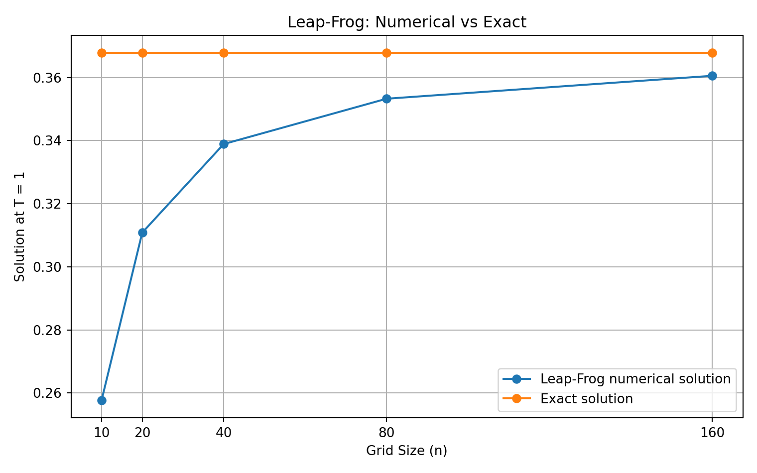
Figure 3. T=1에서 격자 수에 따른 Leap-Frog 근삿값과 정확한 해의 비교.

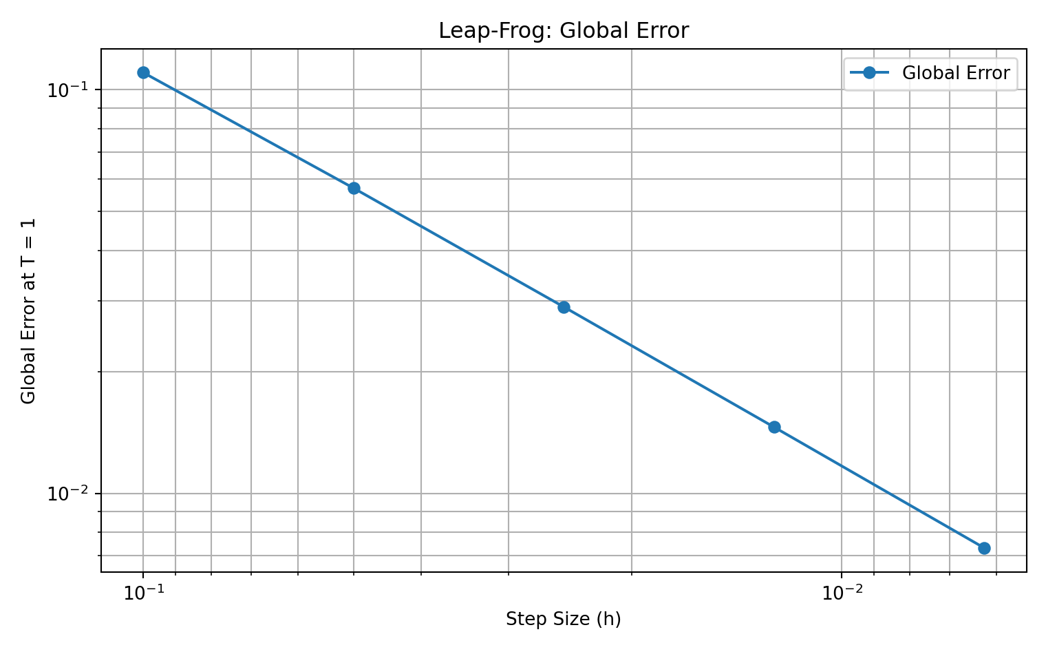
Figure 4. T=1에서 시간 간격 감소에 따른 Global Error.

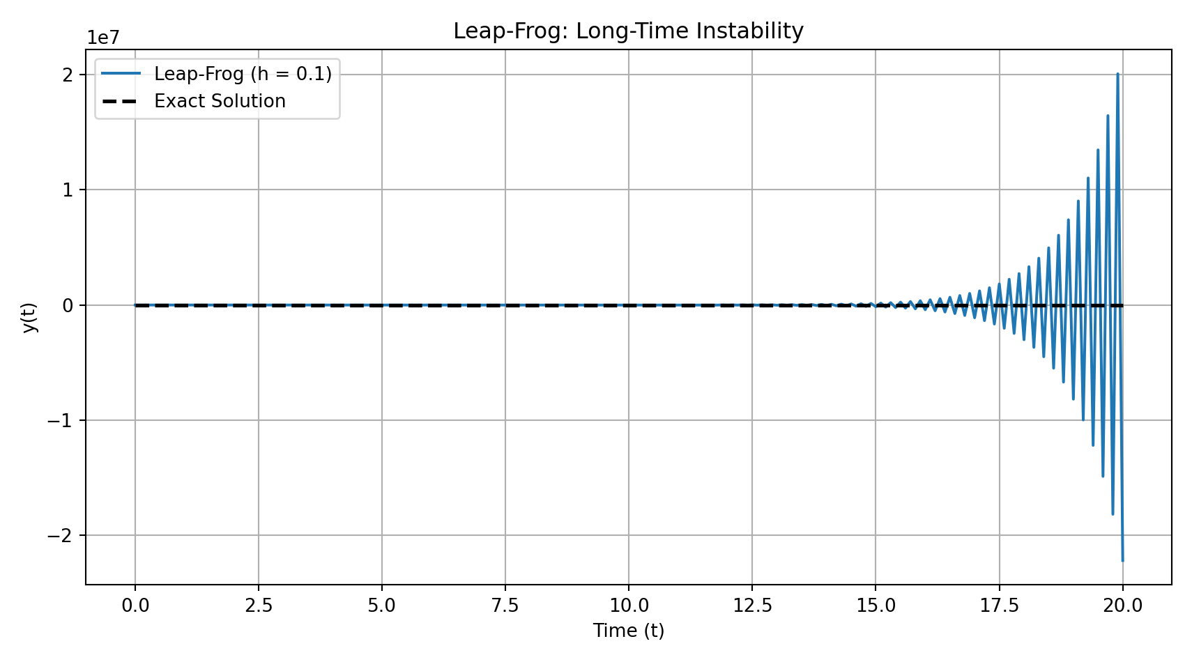
Figure 5. 고정된 h=0.1, T=20에서 Leap-Frog의 불안정한 진동 모드가 성장하는 모습.

Results and Analysis. T=1에서는 n이 커질수록 오차가 감소했다. 그러나 h=0.1로 고정하고 T=20까지 계산하면 정확한 해 e^(−t)는 0으로 감소하는 반면, 수치해에는 커지는 교대 진동이 나타난다. 따라서 이 실험은 짧은 구간에서의 오차 감소가 장기 안정성을 의미하지는 않는다는 점을 보여준다.

또한 Leap-Frog의 매끄러운 정확해에 대한 한 단계 잔차는 2차로 작아지더라도, 두 단계 시작값의 정확도와 특성근에 대한 안정성 조건을 별도로 검토해야 한다.

Lab Handout Problems — Euler Schemes

9.1 Lab Handout Exercise 1 — Forward Euler with Negative Growth Rate

문제는 y'=−4y, y(0)=3이고 최종시간은 T=1, 간격은 h=1/n이다.

Forward Euler를 적용하면 다음과 같다.

정확한 해는 y(t)=3e^(−4t)이다. 지수함수의 극한 공식에서 (1−4/n)^n → e^(−4)이므로 n → ∞에서 수치해가 y(1)=3e^(−4)로 수렴한다. 다만 작은 n에서는 증폭인자 1−4h가 음수이거나 절댓값이 클 수 있으므로 수렴 극한과 개별 시간 간격의 안정성은 구분해야 한다.

9.3 Lab Handout Exercise 3 — Backward / Implicit Euler

문제는 y'=5y, y(0)=2, T=1이다. Backward Euler는 다음 시간의 미지값 yₙ₊₁에서 변화율을 평가한다.

업데이트식이 yₙ₊₁ = yₙ/(1−5h)로 정리되므로 단계를 반복하면 위의 식을 얻는다. 정확한 해는 2e^(5t)이며 n → ∞에서 yₙ → 2e^5이다. 단, n=5이면 분모가 0이 되어 스킴이 정의되지 않는다. 극한을 다룰 때는 충분히 큰 n을 고려한다.

Important Note — Zero-Stability vs Long-Time Instability

Leap-Frog의 근 r₋=−h−√(1+h²)는 고정된 h>0에서 절댓값이 1보다 커 장기적으로 기생 모드가 증폭될 수 있다. 그러나 Zero-Stability를 판정하는 다항식은 h→0의 ρ(ξ)=ξ²−1이며 근 ±1이 단순근이므로 Zero-Stability 자체는 만족한다. 따라서 유한한 시간 구간의 h→0 수렴과 고정 h에서의 장기 불안정을 혼동해서는 안 된다. 상세한 Root Condition은 Post 4에서 다룬다.

Further Validation — Lab 2

Lab 1에서 확인한 세 가지 개념을 Lab 2에서 다시 검증한다. 같은 초기값 문제를 사용하지만, 두 번째 실습은 국소절단오차의 절댓값, 로그 척도에서의 수렴차수, Leap-Frog의 두 특성근과 불안정 모드의 증폭을 더 분명히 드러낸다. 아래 출력 수치는 제출한 LAB_2.ipynb에 저장된 결과이다.

Lab 2 — Exercise 1: LTE and Consistency

Source: Lab-2.pdf, Exercise 1; Lec-2_3_scheme.pdf, Euler Method

y′ = −y, y(0) = 1에서 y(x) = exp(−x)를 이용한다. 고정된 x = 1에서 n = 10, 100, 1000, 10000으로 그리드를 세분화하면 LTE의 절댓값이 감소한다. 1차 일치성이 의미하는 것은 h → 0에서 미분방정식의 잔차가 사라진다는 사실이지, 이것만으로 모든 수치해가 수렴한다는 뜻은 아니다.

Python Implementation

import numpy as np
import matplotlib.pyplot as plt

# Exercise 1: Forward Euler LTE and Consistency

# Fixed evaluation point
x_n = 1.0
n_values = [10, 100, 1000, 10000]

h_values = []
lte_values = []

# Calculate LTE using the exact solution y(x) = exp(-x)
for n in n_values:
    h = 1 / n
    x_prev = x_n - h
    y_n = np.exp(-x_n)
    y_prev = np.exp(-x_prev)

    # Residual LTE for Forward Euler applied to y' = -y
    lte = (y_n - y_prev) / h + y_prev
    h_values.append(h)
    lte_values.append(abs(lte))
    print(f"n = {n:5d}, h = {h:.5f}, |LTE| = {abs(lte):.10f}")

plt.figure(figsize=(7, 5))
plt.loglog(h_values, lte_values, 'o-', label='Absolute LTE')
plt.loglog(h_values, np.exp(-x_n) * np.array(h_values) / 2,
           '--', label='Reference: exp(-1) h / 2')
plt.xlabel('Step size (h)')
plt.ylabel('Absolute LTE')
plt.title('Exercise 1: Forward Euler Consistency')
plt.legend()
plt.grid(True, which='both')
plt.tight_layout()
plt.show()

실행 결과

n =    10, h = 0.10000, |LTE| = 0.0196674740
n =   100, h = 0.01000, |LTE| = 0.0018517060
n =  1000, h = 0.00100, |LTE| = 0.0001840624
n = 10000, h = 0.00010, |LTE| = 0.0000183952

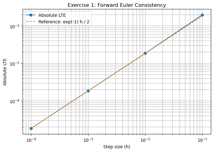
Figure. Lab 2 — Exercise 1: LTE and Consistency (1/1).

Lab 2 — Exercise 2: Empirical Convergence Order

Source: Lab-2.pdf, Exercise 2; Lec-2_3_scheme.pdf, Convergence

y′ = −2y, y(0) = 1의 정해는 exp(−2t)이다. T = 1에서 전역오차를 측정하고 ln(Error)와 ln(h)의 선형 회귀 기울기를 추정한다. 저장된 결과는 p = 1.0106으로, Forward Euler의 이론적 1차 전역 수렴과 일치한다.

Python Implementation

import numpy as np
import matplotlib.pyplot as plt

# Exercise 2: Forward Euler Global Convergence and Order

T = 1.0
n_values = [10, 20, 40, 80, 160]

# Exact solution to y' = -2y, y(0) = 1
def exact_solution(x):
    return np.exp(-2 * x)

# Forward Euler scheme
def forward_euler(y0, T, n):
    h = T / n
    x = np.linspace(0, T, n + 1)
    y = np.zeros(n + 1)
    y[0] = y0
    for i in range(n):
        y[i + 1] = y[i] + h * (-2 * y[i])
    return x, y, h

h_values = []
error_values = []

for n in n_values:
    x, y, h = forward_euler(1.0, T, n)
    error = abs(exact_solution(T) - y[-1])
    h_values.append(h)
    error_values.append(error)
    print(f"n = {n:5d}, h = {h:.5f}, y(T) = {y[-1]:.8f}, Error = {error:.10f}")

# Estimate order from the slope of log(error) vs log(h)
p = np.polyfit(np.log(h_values), np.log(error_values), 1)[0]
print(f"Estimated convergence order p = {p:.4f}")

plt.figure(figsize=(7, 5))
plt.loglog(h_values, error_values, 'o-', label='Global error at T = 1')
plt.loglog(h_values, error_values[0] * np.array(h_values) / h_values[0],
           '--', label='Reference: O(h)')
plt.xlabel('Step size (h)')
plt.ylabel('Absolute global error')
plt.title('Exercise 2: Forward Euler Global Convergence')
plt.legend()
plt.grid(True, which='both')
plt.tight_layout()
plt.show()

실행 결과

n =    10, h = 0.10000, y(T) = 0.10737418, Error = 0.0279611008
n =    20, h = 0.05000, y(T) = 0.12157665, Error = 0.0137586286
n =    40, h = 0.02500, y(T) = 0.12851216, Error = 0.0068231267
n =    80, h = 0.01250, y(T) = 0.13193781, Error = 0.0033974778
n =   160, h = 0.00625, y(T) = 0.13364007, Error = 0.0016952153
Estimated convergence order p = 1.0106

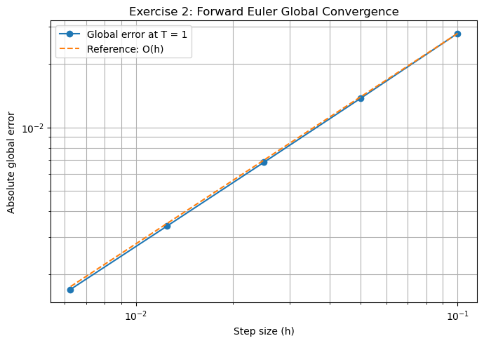
Figure. Lab 2 — Exercise 2: Empirical Convergence Order (1/1).

Lab 2 — Exercise 3: Leap-Frog and the Parasitic Mode

Source: Lab-2.pdf, Exercise 3; Lec-2_3_scheme.pdf, Leap-Frog

y[n+1] = y[n−1] − 2h y[n], y[0] = y[1] = 1에서 특성근은 −h ± sqrt(1+h²)이다. 고정된 짧은 종점 T = 1에서 h를 줄이면 출력된 전역오차가 작아지지만, 고정된 h로 오래 적분하면 절댓값 1보다 큰 음의 근에 대응하는 parasitic mode가 증폭된다. 따라서 이 장기 불안정성과 유한 시간 구간에서의 수렴을 구분해야 한다.

Python Implementation

import numpy as np
import matplotlib.pyplot as plt

# Exercise 3: Consistency Does Not Imply Convergence (The Leap-Frog Trap)

# Final time
T = 1.0

# Number of grid intervals
n_values = [10, 20, 40, 80, 160]

# Exact solution y(x) = exp(-x)
def exact_solution(x):
    return np.exp(-x)

# Leap-Frog method
def leap_frog(y0, y1, T, n):
    h = T / n
    x = np.linspace(0, T, n + 1)
    y = np.zeros(n + 1)

    # Initial values
    y[0] = y0
    y[1] = y1

    # Leap-Frog scheme
    for i in range(1, n):
        y[i + 1] = y[i - 1] - 2 * h * y[i]

    return x, y, h

# Lists to store results
h_values = []
lte_values = []
error_values = []

# Plot 1: Numerical solutions
plt.figure(figsize=(8, 5))

for n in n_values:
    x, y, h = leap_frog(1.0, 1.0, T, n)

    # Exact solution
    y_exact = exact_solution(x)

    # Local truncation error at x = T - h
    lte = ((exact_solution(T) - exact_solution(T - 2*h))
           / (2*h) + exact_solution(T - h))

    # Global error at T = 1
    error = abs(y[-1] - y_exact[-1])

    h_values.append(h)
    lte_values.append(abs(lte))
    error_values.append(error)

    print(f"n = {n:5d}, h = {h:.5f}, "
          f"LTE = {abs(lte):.10f}, "
          f"Global Error = {error:.10f}")

    plt.plot(x, y, label=f'n = {n}')

# Exact solution
x_exact = np.linspace(0, T, 1000)
plt.plot(x_exact, exact_solution(x_exact),
         'k--', linewidth=2, label='Exact solution')

plt.xlabel('Time (x)')
plt.ylabel('Solution y(x)')
plt.title('Leap-Frog: Numerical vs Exact Solution')
plt.legend()
plt.grid(True)
plt.tight_layout()
plt.show()

# Plot 2: LTE and global error
plt.figure(figsize=(7, 5))
plt.loglog(h_values, lte_values, 'o-', label='LTE')
plt.loglog(h_values, error_values, 's-', label='Global Error')

plt.xlabel('Step size (h)')
plt.ylabel('Absolute Error')
plt.title('Leap-Frog: Consistency and Global Error')
plt.legend()
plt.grid(True, which='both')
plt.tight_layout()
plt.show()

# Plot 3: Growth of the oscillatory computational mode
n = 10
h = T / n
x = np.linspace(0, T, n + 1)

# Characteristic roots
r_plus = -h + np.sqrt(1 + h**2)
r_minus = -h - np.sqrt(1 + h**2)

# Coefficient determined by y0 = y1 = 1
B = (1.0 - r_plus) / (r_minus - r_plus)

# Actual oscillatory component
k = np.arange(n + 1)
oscillatory_mode = B * r_minus**k

plt.figure(figsize=(7, 5))
plt.plot(x, oscillatory_mode, 'o-',
         label='Oscillatory Mode')
plt.plot(x, np.abs(oscillatory_mode), '--',
         label='Mode Amplitude')

plt.xlabel('Time (x)')
plt.ylabel('Mode Value')
plt.title('Leap-Frog: Oscillatory Mode Amplification')
plt.legend()
plt.grid(True)
plt.tight_layout()
plt.show()

print(f"\nUnstable root: {r_minus:.6f}")
print(f"Initial mode amplitude: {abs(B):.6f}")
print(f"Final mode amplitude: {abs(oscillatory_mode[-1]):.6f}")
print(f"Amplification factor: {abs(r_minus)**n:.4f}")

실행 결과

n =    10, h = 0.10000, LTE = 0.0006779550, Global Error = 0.1102517932
n =    20, h = 0.05000, LTE = 0.0001611622, Global Error = 0.0570360863
n =    40, h = 0.02500, LTE = 0.0000392921, Global Error = 0.0289614969
n =    80, h = 0.01250, LTE = 0.0000097008, Global Error = 0.0145869868
n =   160, h = 0.00625, LTE = 0.0000024101, Global Error = 0.0073194539

Unstable root: -1.104988
Initial mode amplitude: 0.047270
Final mode amplitude: 0.128281
Amplification factor: 2.7138

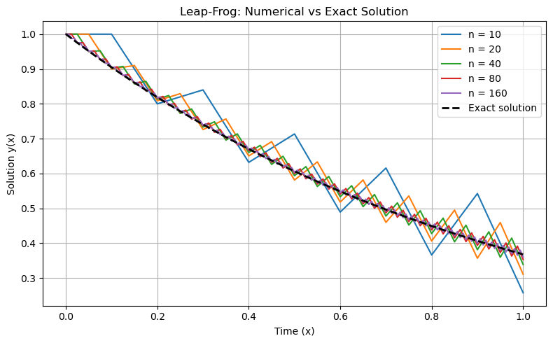
Figure. Lab 2 — Exercise 3: Leap-Frog and the Parasitic Mode (1/3).

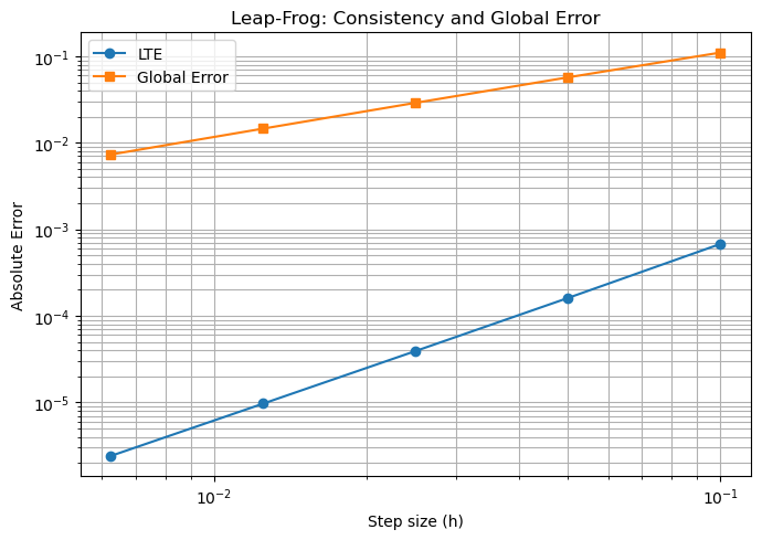
Figure. Lab 2 — Exercise 3: Leap-Frog and the Parasitic Mode (2/3).

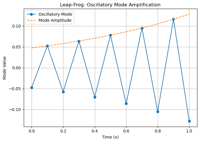
Figure. Lab 2 — Exercise 3: Leap-Frog and the Parasitic Mode (3/3).

Detailed Lecture Notes — Euler Schemes and Convergence Proofs

여기서는 Lec-2_3_scheme.pdf의 Numerical Solutions와 Euler Method 절을 차분 연산자의 정의부터 수렴성 증명의 마지막 상계까지 자세히 다시 계산한다. 기존 Lab 1·2 코드와 그래프는 앞부분에 그대로 유지했다.

8.8 Forward and Backward Difference Operators

격자

에서 도함수의 전진차분과 후진차분을 각각 정의하면

이다. Taylor 정리를 쓰면

이므로

를 얻는다.

에서 남은 고차항을 버리면 Forward Euler

와 Backward Euler

가 나온다.

전진형은 다음

을 바로 계산하는 explicit 방법이고, 후진형은 미지수

가 우변에도 등장하므로 일반적으로 각 단계에서 비선형 방정식을 풀어야 하는 implicit 방법이다.

8.9 Local Truncation Error: Two Normalizations

강의에서는 미분방정식 잔차로 정의한 LTE를 사용한다. 정확해를 수치방정식에 넣어

이라고 하면 Taylor 전개로

이므로

에서 0으로 가서 consistent이다. 한편 한 단계 업데이트의 결손량을

이라고 정의하면

이다. 따라서 ‘Euler LTE는

‘와 ‘한 단계 오차는

‘라는 진술은 **오차를

로 나누는지에 따라 동시에 맞을 수 있다**. Lab 코드에서 사용한 LTE 정의를 확인해야 비교가 가능하다.

주의 — Lecture의 인쇄식: 원본은 Taylor 전개의 평가점과 잔여항 차수 표기가 혼동될 수 있으므로, 위 유도는 **정확해를

에서 전개하는 표준 표기**로 명시했다. 강의의 결론인 consistency와 1차 수렴성은 유지된다.

8.10 Global Convergence: Full Induction Argument

정확해와 수치해의 차이를

로 정의한다. 초기값을 정확히 지정했다고 가정하여

이다.

라고 하자.

Taylor 전개에 의해

이고, Euler 수치식

를 빼면

이다.

가 상태변수에 대해 Lipschitz이면

이다.

라고 놓고 귀납적 반복을 수행하면

이며 등비수열 합을 계산해

이다.

이므로

일 때

를 얻는다.

인 경우에는 따로

로 처리한다. 따라서 Forward Euler는 고정 구간에서 1차 수렴한다. 강의 Theorem 2.3은 Forward·Backward Euler 두 방법 모두 1차 수렴한다고 기술하고, 증명은 Forward Euler에 한정해 제시한다. 여기서도 그 범위를 구분했다.

8.11 Estimating Convergence Order from a Table

전역오차가

이면

이므로 양변에 로그를 취해

를 얻는다. 예를 들어 표를 만들 때

를 절반으로 줄였더니 오차도 절반으로 줄어들면

, 오차가 네 배 줄면

라고 읽는다. Notebook의 회귀 기울기는 여러

값에 대해

를

에 선형회귀한 것으로, 같은 원리다.

8.12 Leap-Frog: Characteristic Equation and Parasitic Root

강의는 다음 두 단계 점화식을 사용한다.

이는

를 중앙차분으로 근사한 것이다. 정확해를 넣어 계산한 미분형 LTE는

이므로 일관성이 있다. 그러나 일반해

을 대입하면

이고,

에서

이다. 따라서 고정된 시간 간격으로 무한히 오래 전진하면

성분이 증폭되는 parasitic mode가 존재한다.

일반해는

이고 시작값으로

을 얻는다. 따라서

이다.

이므로 이 시작값에서는

로 작지만 0은 아니다. 중요한 구분: 유한한 고정 시간

에서

인 수렴 문제와,

를 고정하고

인 장기 안정성 문제는 다르다.

만 보고 ‘모든 고정시간에서

수렴하지 않는다’라고 결론 내릴 수는 없다. 원본 강의는 이 차이를 엄밀히 구별하지 않은 문장을 포함하고, Lab 2의 긴 시간 실험은 장기 불안정성을 보여주는 자료로 해석하는 것이 정확하다.

8.13 Explicit Euler Worked Example: Negative Growth

Lab Handout Exercise 1은

]]이다.

이면

이므로 귀납적으로

이다. 정확해는

이며

이다.

이 작은 경우

이 음수이거나 0일 수 있지만, 극한 계산은

에서 수행한다.

8.14 Backward Euler Worked Example: Positive Growth

Lab Handout Exercise 3은

이다. 후진 Euler는

을 준다(단,

). 정확해

와 비교하면

이므로

일 때

이다. 로그 전개를 쓰려면 충분히 큰

를 가정한다.

8.15 Full Lecture Checklist — Euler Section

이 글에 Numerical Solutions, explicit/implicit Euler, finite differences, LTE 정의, consistency, convergence 정의, First-Order Convergence Theorem, 귀납적 오차증명, Leap-Frog 반례, Taylor 확장으로 넘어가는 논의를 포함했다. Lab 1·2의 그림은 기존 /assets/images/ode_*.png 경로 그대로 사용한다.

Source-by-Source Verification — Euler Lecture and Lab Exercises

Full Taylor Check for the Euler Local Error

강의 p.3의 LTE는 h로 나눈 잔차형 LTE이다. y(t+h)를 t에서 전개하면

반면 한 스텝의 업데이트 오차는 위 식에 h를 곱한 것이므로 O(h²)다. 교수 자료 p.3의 Taylor 표기에 인덱스와 차수의 오탈자로 보이는 부분이 있지만, 원래 과제가 확인하려는 잔차 LTE = O(h), 한 스텝 오차 = O(h²)는 구별해야 한다. 이는 강의 공식과 직접 Taylor 전개를 대조한 검산 결과다.

Fixed-Time Zero Error: Lecture Question

강의 p.4의 질문, Forward Euler에서 모든 n에 대해 오차가 0이 되는 사례가 있는가?의 답은 있다이다. y′=0, y(0)=1이라면 정확해는 y(t)=1이고 Euler 업데이트도 yₙ₊₁=yₙ이므로 모든 격자점에서 정확히 일치한다. 보다 일반적으로 y′=a, y(0)=b와 같이 해가 시간의 일차함수인 경우에도 Euler는 정확하다.

Leap-Frog: What the Root Calculation Actually Proves

강의 p.3의 고정된 h>0에 대한 근은 다음과 같다.

그러므로 일반적인 초기화에서 기생모드가 고정된 h로 장시간 적분할 때 커진다. 하지만 h→0, nh=T 고정인 수렴 문제와 혼동하면 안 된다. h=0의 첫 특성다항식은 ρ(r)=r²−1이며 두 단위근 +1,−1은 서로 다른 단순근이다. 따라서 이 방법은 고전적 의미의 zero-stability 조건을 충족한다. y₀=y₁=1이라는 초기화는 정확한 y(h)=e^(−h)와 O(h)만큼 다르므로, 고정된 T에서 수렴하더라도 초기화 때문에 관측 차수가 낮아질 수 있다. 이 점은 Lab-2의 T=1 및 장기 그래프를 함께 해석할 때 필수다. 강의의 ‘lack of convergence’ 문장은 일반적인 장기 성장 현상을 강조한 것으로 읽되, 모든 고정 T에서 h→0 수렴 불가능하다는 결론으로 확대하지 않는다.

Handout Exercise 1 and Exercise 3: Closed Forms and Limits

y′=−4y, y(0)=3, h=1/n인 Forward Euler는 yₙ₊₁=(1−4/n)yₙ, 따라서

y′=5y, y(0)=2인 Backward Euler는 yₙ₊₁=yₙ+(5/n)yₙ₊₁이므로 n≠5에서

단, n=5이면 첫 암시적 방정식을 유일하게 풀 수 없다. n<5에서는 단계 계수가 음수일 수도 있으며, 극한을 증명할 때에는 n>5의 충분히 작은 스텝 크기를 고려한다. 이 예외를 무시한 무조건적인 닫힌형 공식은 부정확하다.

Consistency는 국소 오차가 사라진다는 조건이고, Convergence는 실제 해에 접근한다는 조건이다. Leap-Frog는 작은 LTE만으로 충분하지 않다는 사실을 보여 준다. Long-time Instability의 원인은 Post 4의 Root Condition과 연결해 다시 정리한다.

References

• Raj Dhara, Lec-2_3_scheme, 2026-10-12, pp. 1–4.
• Raj Dhara, Numerical Method Lab: ODE Numerical Schemes & Convergence, Exercises 1 and 3.
• LAB_1.ipynb, Exercises 1–3 (Python implementation and stored results).

---